How to hide unused cells in Excel

There are many reasons you might need to hide unused cells. One of the reasons could be that you need to focus on a particular part or data range. If you keep getting distracted, your work will not be effective and efficient. 

So, do you want to know how to hide unused cells in Excel? Don’t worry, We got you. We can hide unused cells in 3 simple steps. I will show you how to hide unused cells in Excel in 3 ways. 

We can hide unused cells from/using:

1. Right-click on the mouse.
2. From the “Format” section.
3. Using a shortcut. 

But first, what are the steps to hide unused cells? 

There are three steps:

• Select the unused data range or columns or rows.
• Choose a method to hide the data.
• Hide the data range. 

How to Select Unused Cells in Excel

Step 1: Select the unused cells. How can we select the unused cells? Well, one thing we need to clear out first. Unused cells means it contains both rows and columns. So, we need to select columns and rows first and then hide them.

Let us take a look at our data first. 

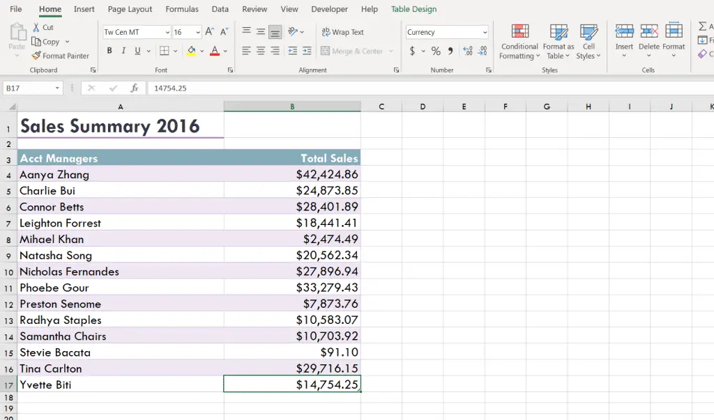
We can see that there is data from rows 1 to 17 and columns A to B. So, the rest of the columns and rows are unused. So, we want to hide these columns and rows. 

To select a single row: 

• Select any cell in that row > Press “Shift + Spacebar.”
• Or take your mouse to the row number and right-click. 

To select multiple or contiguous rows: 

• Select any cell in that row >  Press “Shift + Spacebar” > Press  “Ctrl + Shift + Down Arrow.” If the unused cells or rows are on the up, then “Ctrl + Shift + Up Arrow.”
• Or take your mouse to the row number and right-click> Press  “Ctrl + Shift + Down Arrow.” If the unused cells or rows are on the up, then “Ctrl + Shift + Up Arrow.”

To select a single column: 

• Select any cell in that column > Press “Ctrl + Spacebar.”
• Or take your mouse to the column number and right-click> Press “Shift + Spacebar.” 

To select multiple or contiguous rows: 

• Select any cell in that column >  Press “Ctrl + Spacebar” > Press  “Ctrl + Shift + Right Arrow.” If the unused cells or columns are on the left, then “Ctrl + Shift + Left Arrow.”
• Or take your mouse to the column number and right-click> Press  “Ctrl + Shift + Right Arrow.” If the unused cells or columns are on the left, then “Ctrl + Shift + Left Arrow.”

Now, we will select the rows and columns and see how we can hide these. 

Whether we select single or multiple rows or columns, the method is the same for hiding rows or columns. So, we are going to select multiple rows or columns. 

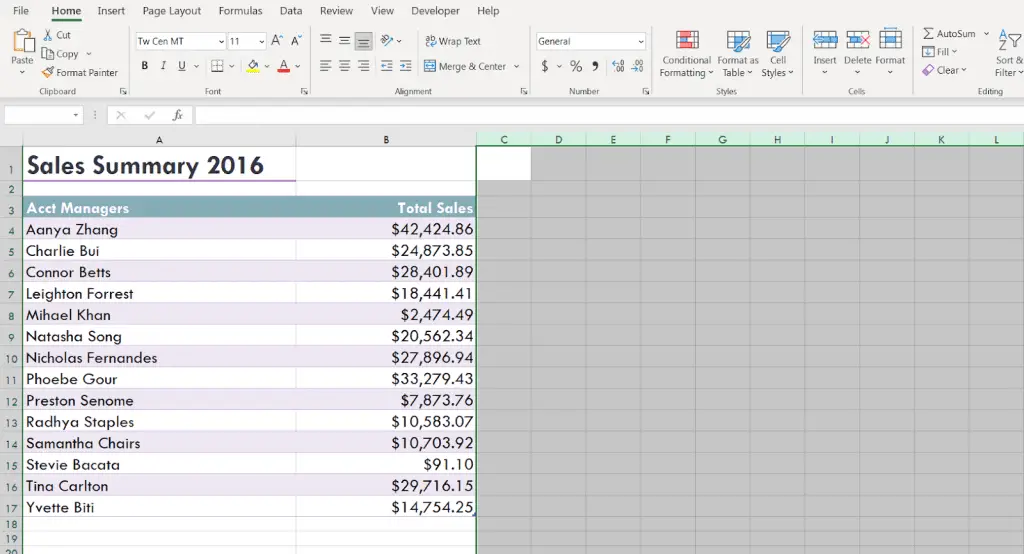
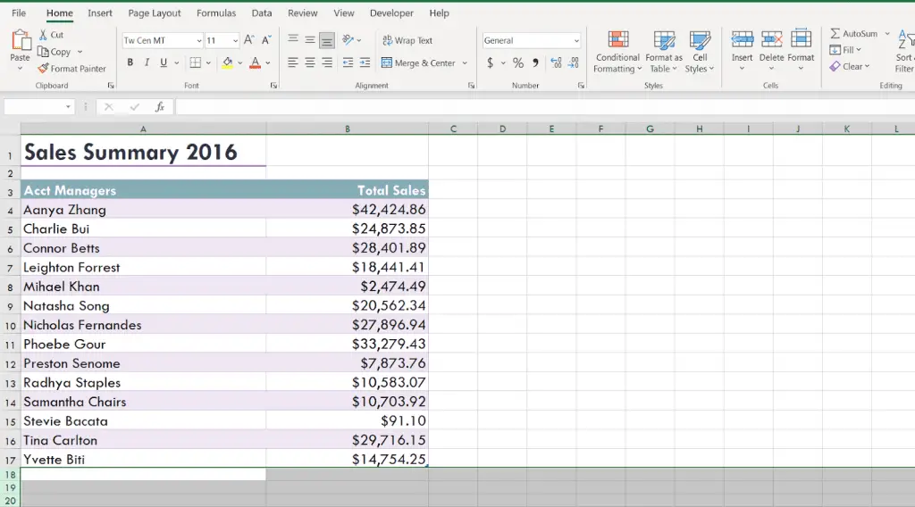
Let us look at how it looks after selecting the rows or columns.

Column: 

Rows: 

After selecting the data range, now is the time to hide the unused rows or columns. 

Step 2: Choose a method to hide. (Right-click / Format Section / Shortcut)

In this section, we will hide the data rows or columns. 

How to Hide Unused Cells in Excel Using Right Click

After selecting the rows and columns, right-click on the mouse. 

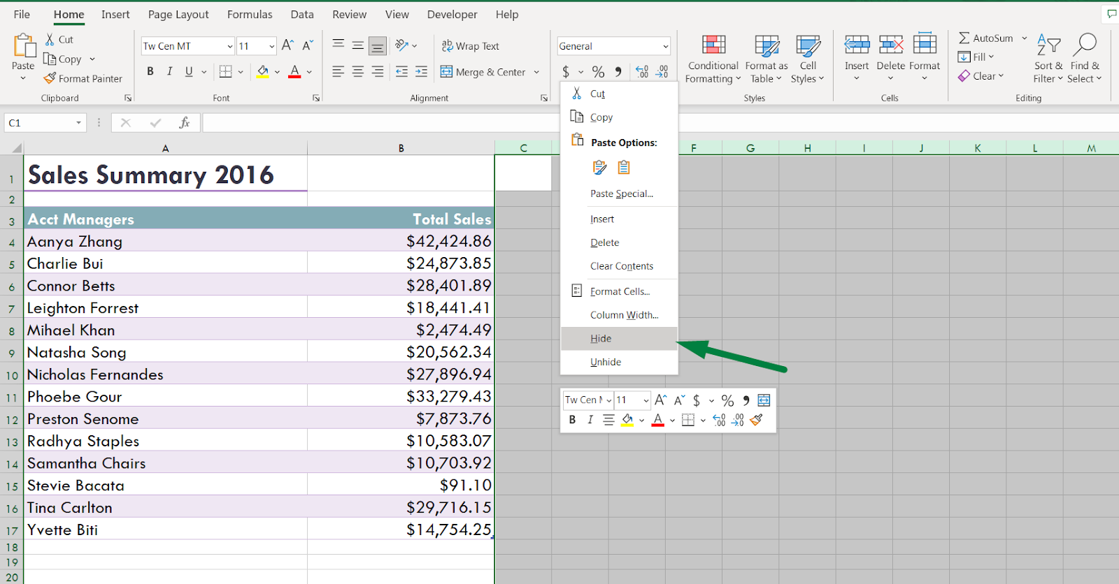
 A box will pop up like this. You will find an option named “Hide.” Click on that.  Whether you select columns or rows, excel will hide those data ranges. 

How to Hide Unused Cells in Excel Using the  “Format” Section

After selecting the rows or columns, go to the “Home” ribbon. Click on the “Format” option under the “Cells” section. 

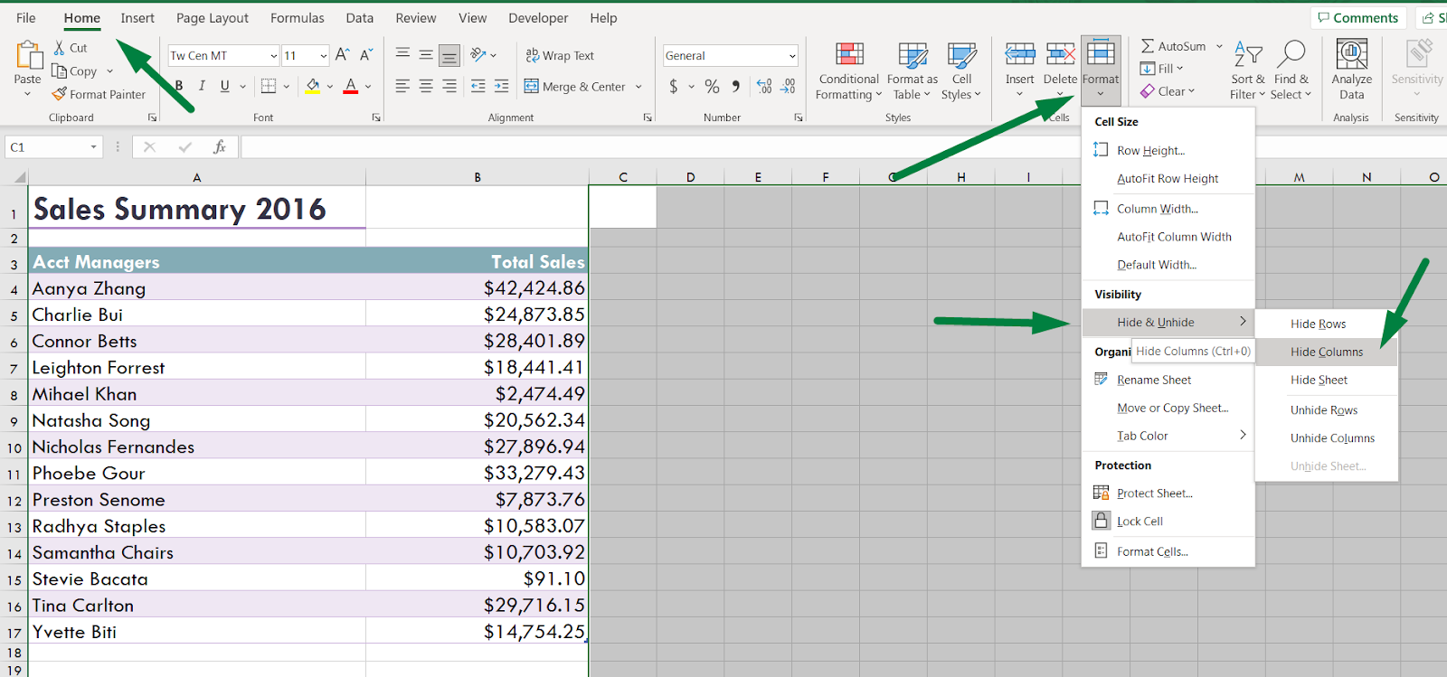
A drop-down menu will come down like this. Under the “Visibility” option, another option is “Hide or Unhide”. Go to that option.

To hide the columns of the selected cells, click “Hide Columns.” 

A shortcut:

To hide unused columns:

After selecting the columns, press “Ctrl + 0 (Zero)”.

Now, we want to hide the rows which contain unused cells. 

So, we are going to select the rows. 

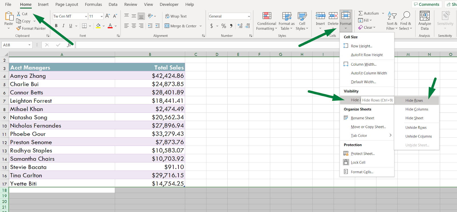
Go to the “Home” ribbon. Click on the “Format” option under the “Cells” section. 

A drop-down menu will come down like this. Under the “Visibility” option, another option is “Hide or Unhide”. Go to that option.

To hide the columns of the selected cells, click “Hide Rows”. 

A shortcut:

To hide unused rows:

After selecting the columns, press “Ctrl + 9 (Nine)”.

How to Hide Unused Cells in Excel Using Shortcut

We can also use the same format section to hide unused cell rows or columns. 

To hide unused columns, use a shortcut:

After selecting the columns, press “Alt + H + O + U + R”

To hide unused rows, use a shortcut:

After selecting the rows, press “Alt + H + O + U + R”

So, we can also use this shortcut to hide unused cells. 

Summary

To summarize all that: 

The easiest way to hide unused cells in Excel:

For columns: Select a single column or multiple columns > press “Ctrl + 0 (Zero)”.

For rows: Select a single column or multiple columns > press “Ctrl + 9 (Nine)”.

Besides this method, after selecting the data,

• Right-click on the mouse > Hide
• Home ribbon > Format option > Hide and unhide > Hide Rows/Columns.
• Press “Alt + H + O + U + R” (For rows) and “Alt + H + O + U + C” (For columns).

So, we tried to cover most of the things on this topic. Let us know in the comment section what else you want to know.