How to Show Gridlines in Google Sheets (In 3 Clicks)

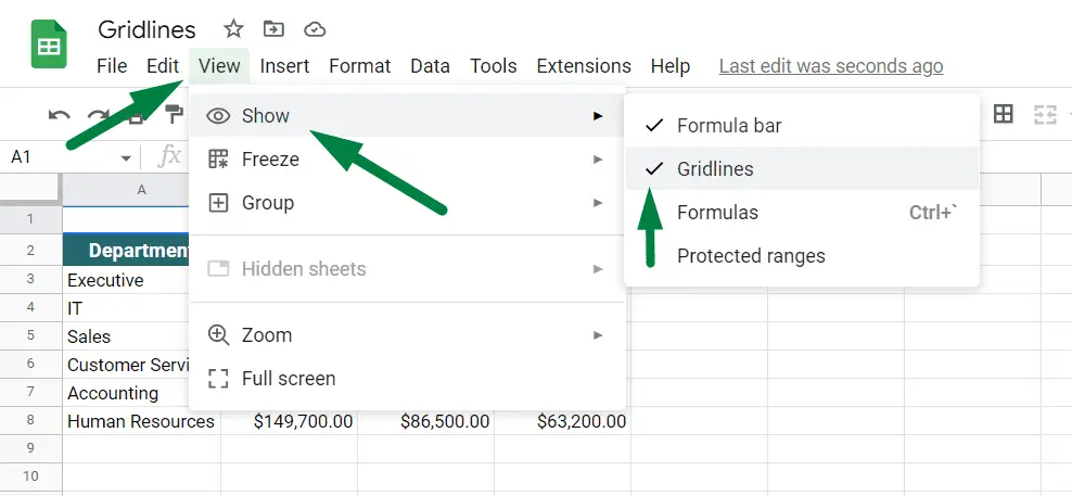
You can show gridlines in Google Sheets by clicking on the “View” tab, putting the mouse cursor in the show option, and ensuring that there is a tick mark beside the “Gridlines” option.

Gridlines make the difference in the worksheets while seeing the content in those columns or rows. Sometimes you might need to hide the gridlines in the Google sheet. 

But you can always add the gridlines to your worksheet.

We will learn how to show gridlines in google sheets within a few steps. Stay with us to learn more.

How to Show Gridlines in Google Sheets (Step-by-Step)

Let’s see how we can add gridlines in google sheets within just three clicks. 

Click on the ‘View’ ribbon > Navigate your cursor to the “Show” option > Mark or Tick the ‘Gridlines’ option. It will show the gridlines in the Google sheet.

See? We can easily add or remove gridlines in Google Sheets. 

Note: You can only show gridlines in your worksheet one at a time. You can’t add gridlines in multiple worksheets in Google Sheets as we can in excel.

In the same way, we can also show and remove gridlines in Excel. 

How Do You Add Gridlines to A Graph In Google Sheets?

Gridlines in a graph are essential as well. You might need to add gridlines to your graphs to visualize and understand the data point and make the chart more readable. 

First, you need to open the gridlines option to add gridlines to a graph. 

Way 1: Double-click on the graph > This will open the “Chart Editor” option.

Way 2: Right-click on the chart > Select the “Gridlines and ticks” option > Click on the Vertical Axis.

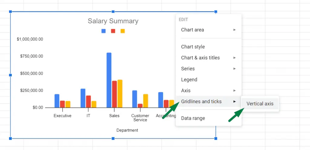
This will also open the “Chart Editor” option with the “Customize” tab. From there, you can add vertical gridlines to your graph.

How to Add Vertical Gridlines in Google Sheets

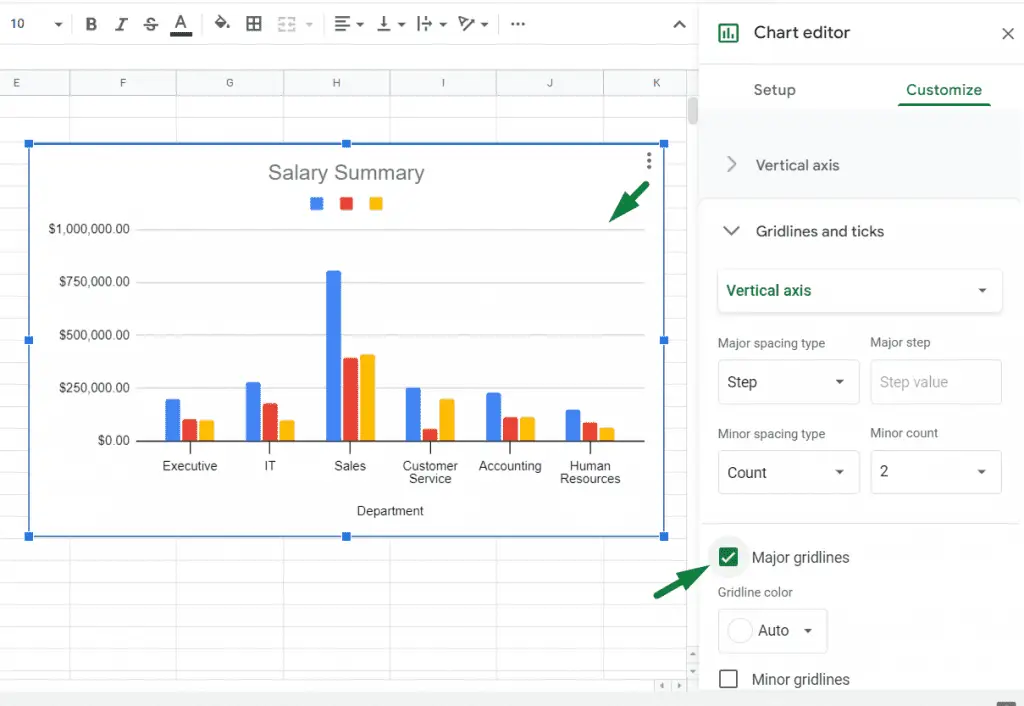
You can add major and minor gridlines under the “Vertical Axis” option.

When you mark or tick the “Major Gridlines” option, the graph will look like this;

And if you mark the “Minor gridlines” option, the graph will look like this. 

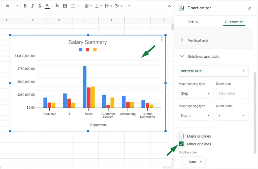
In these ways, you can add vertical major and minor gridlines to your graph. 

There are also options to add major and minor ticks as well. 

Summary

To add gridlines in Google Sheets (In a single worksheet): Click on the ‘View’ ribbon > Navigate through the ‘Show’ option > Mark the ‘Gridlines’ option.

To add gridlines to a graph in Google sheet: 

Way 1: Double-click on the chart > Customize tab > ‘Gridlines and ticks’ option > Select Vertical Axis > Mark the ‘Major’ or Minor gridlines.

Way 2: Right-click on the chart > ‘Gridlines and ticks’ option > Vertical Axis > Mark the ‘Major’ or Minor gridlines.

Conclusion

You can add gridlines to your worksheet and your graphs as well. Within just a few clicks, you can show the gridlines.

Let us know if you have any questions regarding gridlines, excel related problems, or analytics problems. Have a great day!