How to Make A Drop Down List In Excel? (3 Easy Steps)

There are many situations where we need to sort items by category. We might need to put each category name beside those items. Now, it might be very time-consuming to write every category name every time or copy-paste the names. 

The practical solution could be creating a drop-down list. You might be asking how to make a drop down list in excel?

First, select the cells where you want to make a drop-down list. Then go to the “Data” ribbon. Select the “Data Validation” option under the “Data Tools” section. Or press Or press “Alt + A + V + V.” Then, select the “List” option under the “Allow:” option and select the names or lists in the “Source” section. Then click “Ok.”

The previous paragraph is just an overview. We discussed every step and option in this article in detail. 

Stay with us to learn more.

How to Make A Drop Down List In Excel (Step-by-Step)

Creating a drop-down list in excel is easy. You don’t need to know advanced techniques. 

We can learn how to do this in just three steps. Let’s get into it.

Step 1: Select the cells where you want to create a drop-down list

This is our first step. Here we need to select the cells, or the column, or the row where we want to create a drop-down list. 

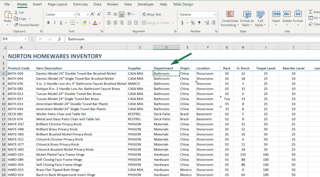
As shown in the picture, we want to create a drop-down list in the D column or Department column. 

Now, as we want to create a drop-down list here, we need to select the cells, or we can just select the whole column. 

To select the column, just click on the column name or the letter “D.” This way, you can learn how to create a drop down list in excel for an entire column. 

Or, to select the cells, select the first cell of that column. Then press the “Ctrl + Shift + Down Arrow (↓)” keys.

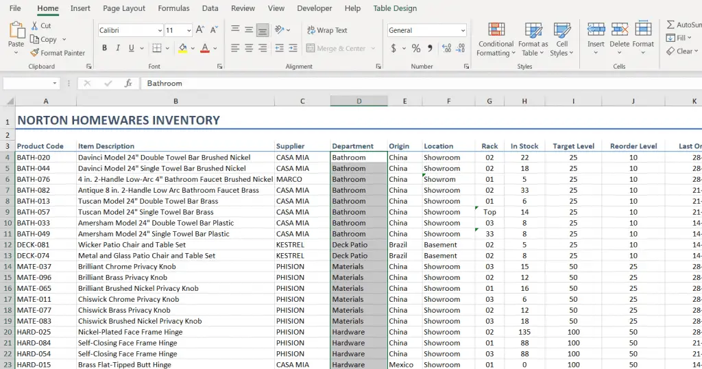
I am going to use this option. 

Step 2: Go to the “Data” ribbon > Select the “Data Validation” option

To create a drop-down list, we need to go to the “Data” ribbon. 

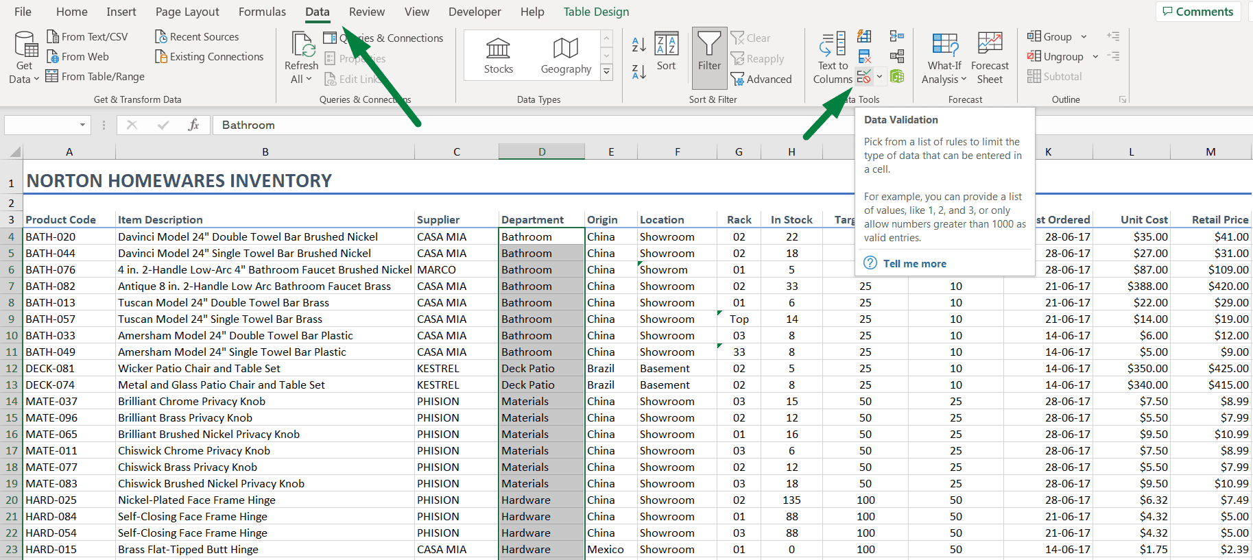
There you will find an option named “Data Validation”. Click on that option. Or you can use the shortcut key to open the data validation box: “Alt + A + V + V.”

This will open a box like this.

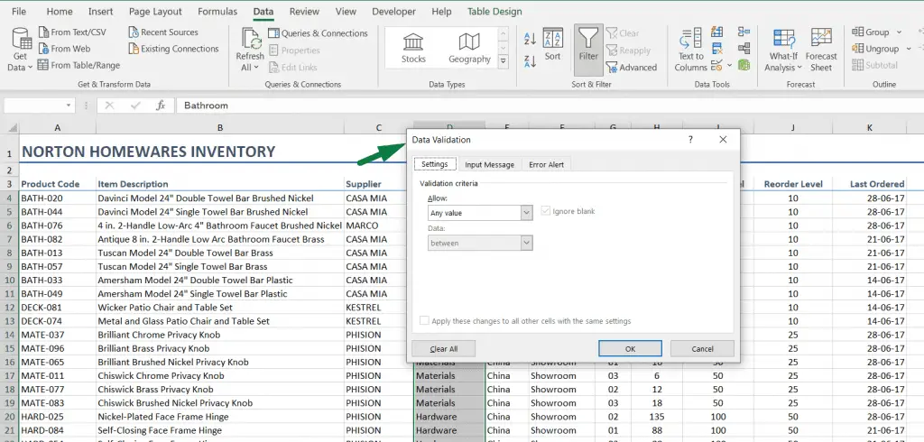
You will find three sections: Settings, input message, and error alert. 

We will learn more about these in another article.

Step 3: Select the names or list or source of the drop-down list

This is the main part where we will learn how to insert the values we want to see in the drop-down list.

But first, click on the down arrow sign under the “Allow:” option. This will show you a range of options. Click on the “List” option. 

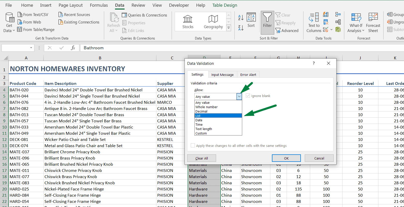
This way, Excel will create a list or drop-down menu by choosing the list option.

But the question is, what will be the values or what will be in the list names? And how are we going to choose that? 

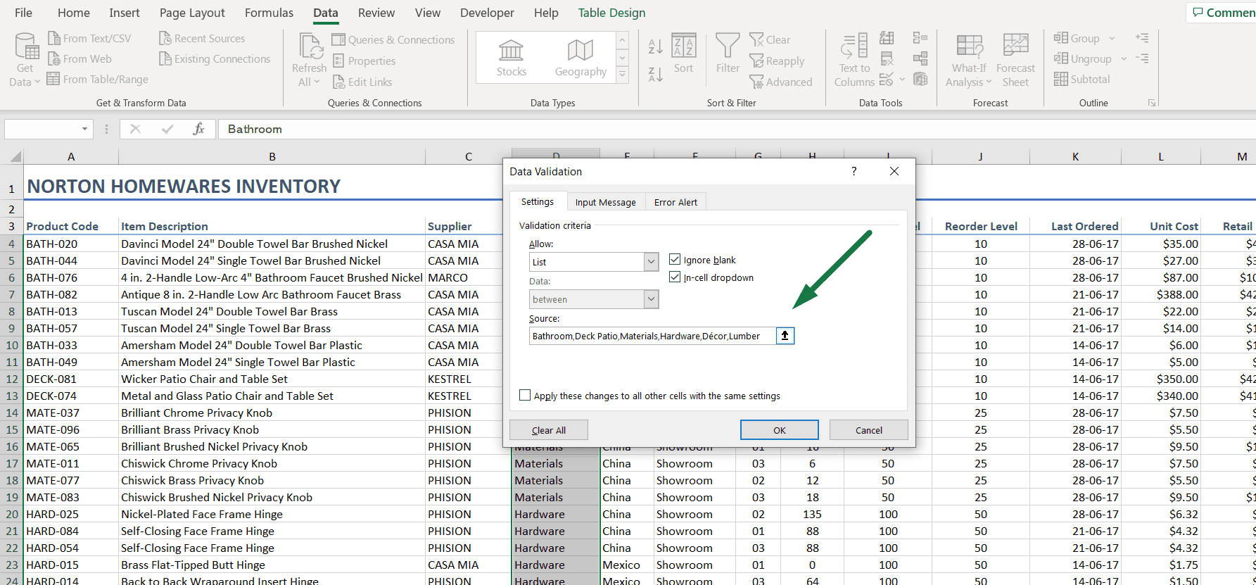
Click on the blank box under the “Source:” option. Now, we can type down all the category names separated by a comma. 

We have six different category names. We will type all the category names separated by a comma, as shown in the screenshot. Then click ok. 

Or we can learn how to create a drop-down list in excel from another sheet.

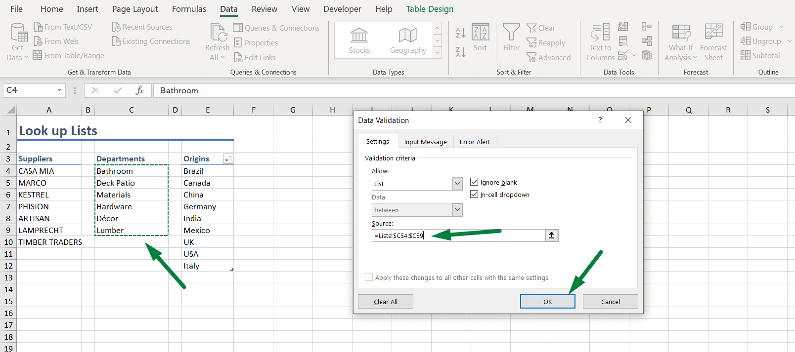
We already have the category name or values name in another sheet, we can select the names from there. And then click ok. 

Now, if we go back to the main sheet, we create the drop-down list. When we select a cell, it will show us the options or values from the list. This is how you can make a drop-down list in excel.

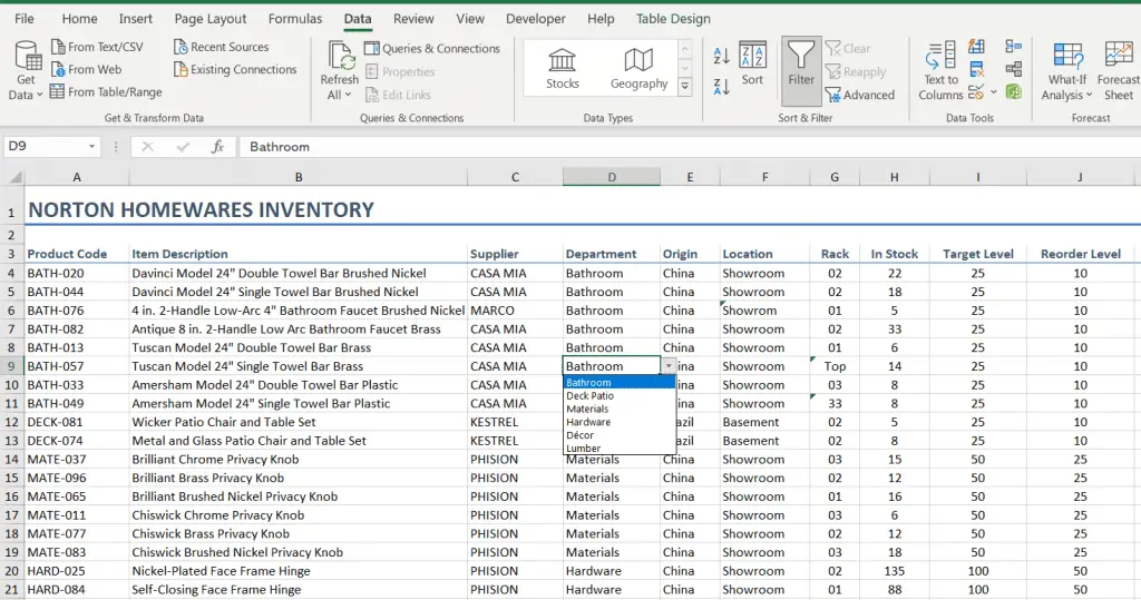
See?  That was easy, right? We can edit or delete the drop-down list if we need to change the sources. 

This way, we can now easily create a drop-down list in excel. 

Summary

We are going to summarize the whole article. Here is an overview of how to make a drop down list in Excel.

1. Select the column or cells where you want to create the drop-down list.
2. Go to the “Data” ribbon. 
3. Click on the “Data Validation” option under the “Data Tools” section.
4. Select the “List” option under the “Allow:” option.
5. Then, type down the values separated by a comma or select the source of the values you want to show in the drop-down list.
6. Click ok.

Shortcut Used

Shortcut to open the data validation box: Alt + A + V + V.

FAQs

How to Create Drop-Down List in Excel 2016?

To create a drop-down list in Excel 2016, select the cells or columns where you want to create a drop-down list. Go to the “Data” ribbon. Select the “Data Validation” option under the “Data Tools” section. Select the “List” option under the “Allow:” option. Select the names or lists in the “Source” section. Click “Ok.”

How to Create a Drop Down List in Excel For an Entire Column?

To create drop-down list in excel for an entire column, click on the column where you want to make the drop-down list. Go to the “Data” ribbon > Select the “Data Validation” option under the “Data Tools” section. Select the “List” option under the “Allow:” option. Select the names or list in the “Source” section. Click “Ok.”

How to Create a Drop Down List in Excel From Another Sheet?

To create a drop-down list in excel from another sheet, select the cells or column where you want to create a list. Go to the “Data” ribbon. Then, select the “Data Validation” option under the “Data Tools” section. Afterward, select the “List” option under the “Allow:” option. And last of all, Click on the blank box of the “Source” section. Go to that sheet where the values you want to show are in the drop-down box. Select those cells. Click “Ok.”

Conclusion

Excel has many great options, making our work easier and more efficient. Such as, we learned how to make a drop down list in excel just in 3 easy steps. 

I hope this article helped you to find solutions to your problems. We wish you all the best!