Find the lowest number in Excel

You can find the lowest number in Excel using the MIN, and SMALL functions. Not to mention, you can also find the lowest number using conditional formatting, combining INDEX, MATCH, and  MIN functions. Lastly, you can also find the lowest number with single or multiple criteria.

Find the lowest number in Excel using the MIN function 

Let’s explain the function first. 

The “Min” function determines the smallest value among a range of numbers. Let’s see how. 

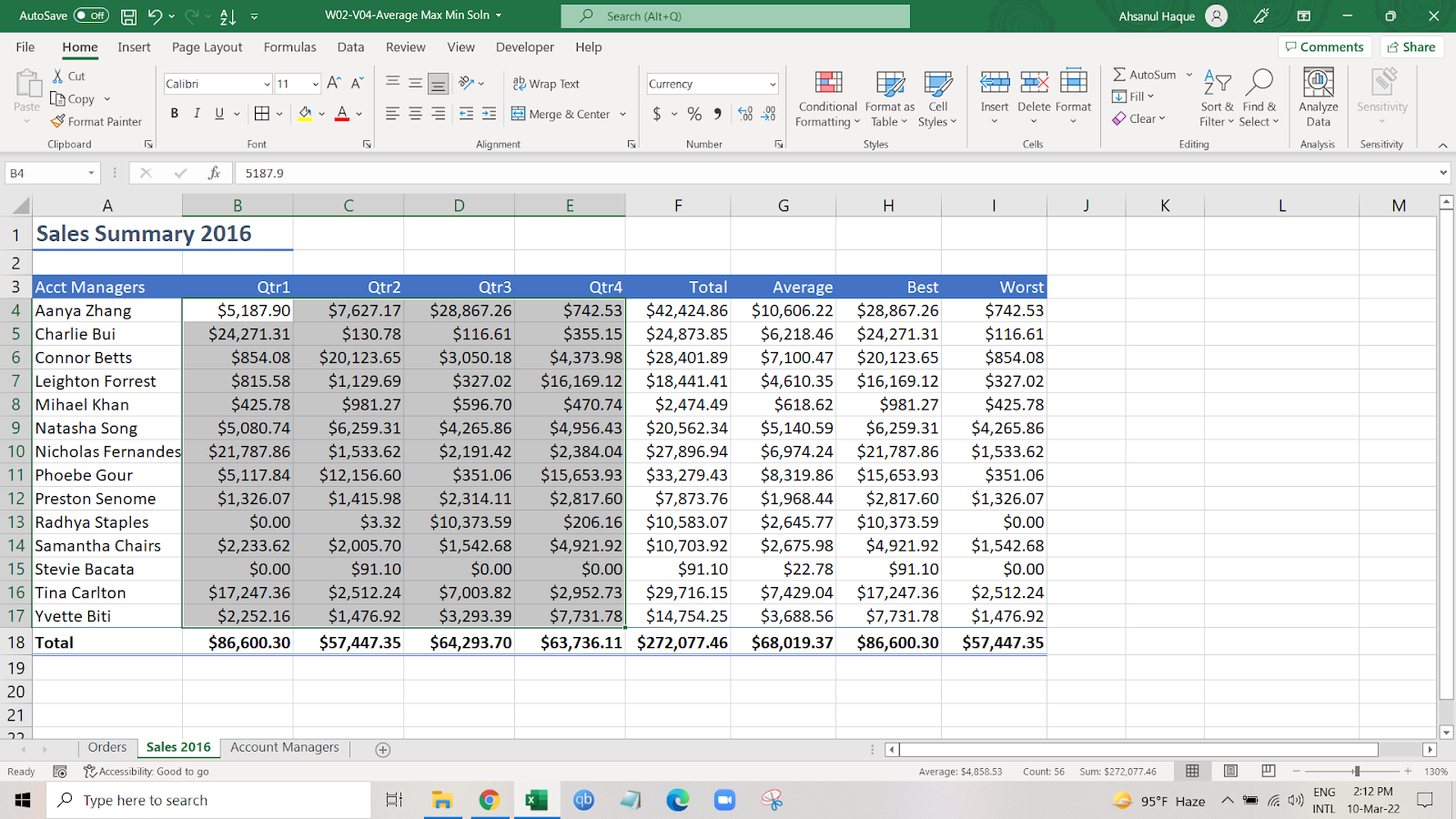
For example, In a company, there are a few account managers. The year is divided into four quarters. 

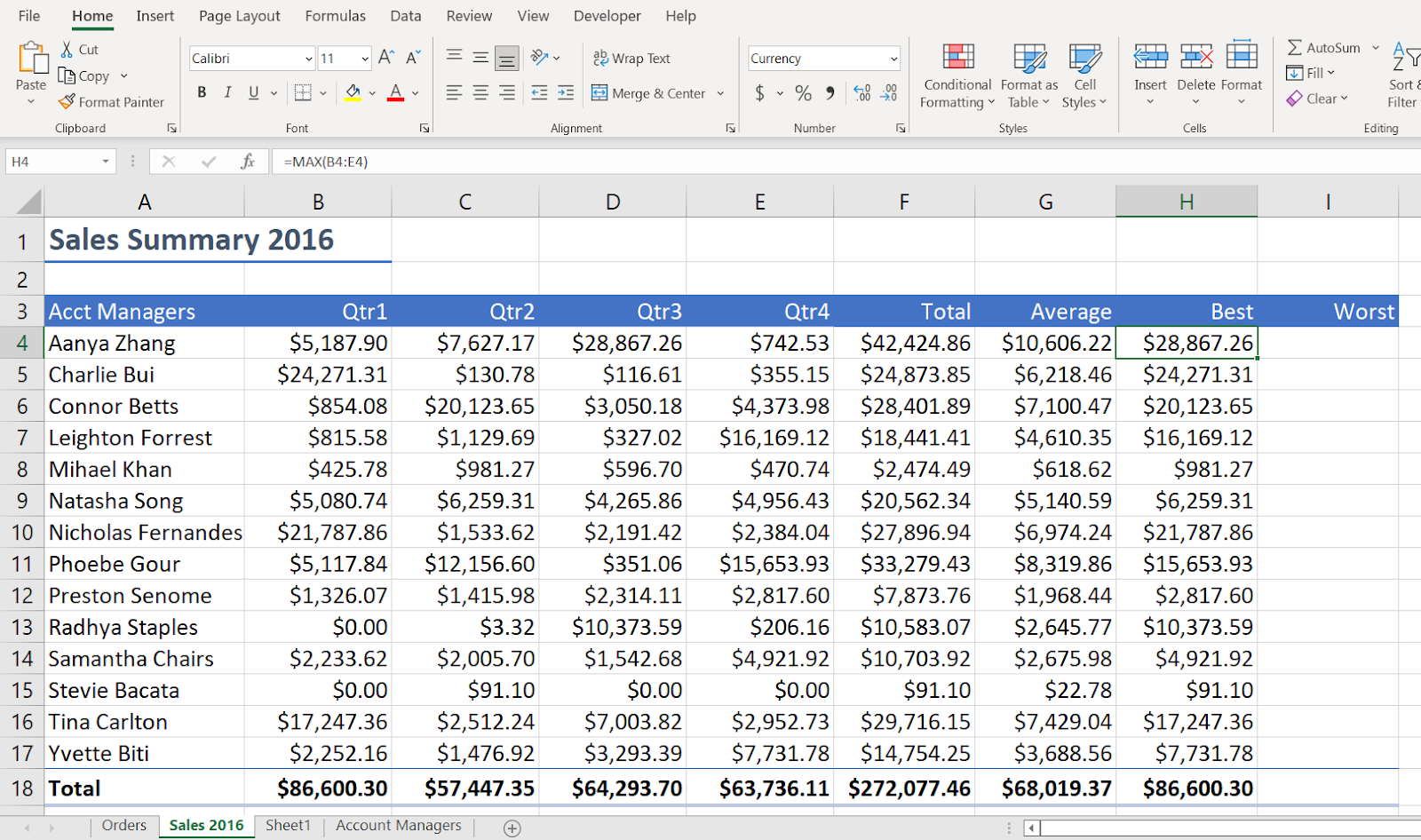
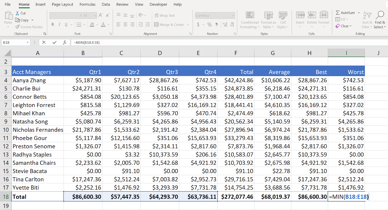
Now, we want to know which was the worst quarter number for each manager. So, we will select the cell where we want to perform the function. 

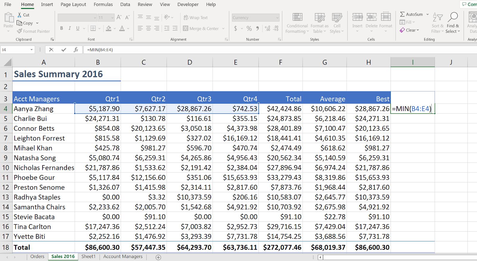
As we want to know the lowest number among the four quarters, in that cell, we put the “Min” function.

A little bit of explanation. 

=MIN(B4:E4)

• Min function because we want to know the lowest number. 
• We selected B4:E4 because we want to know the lowest number among those numbers. 

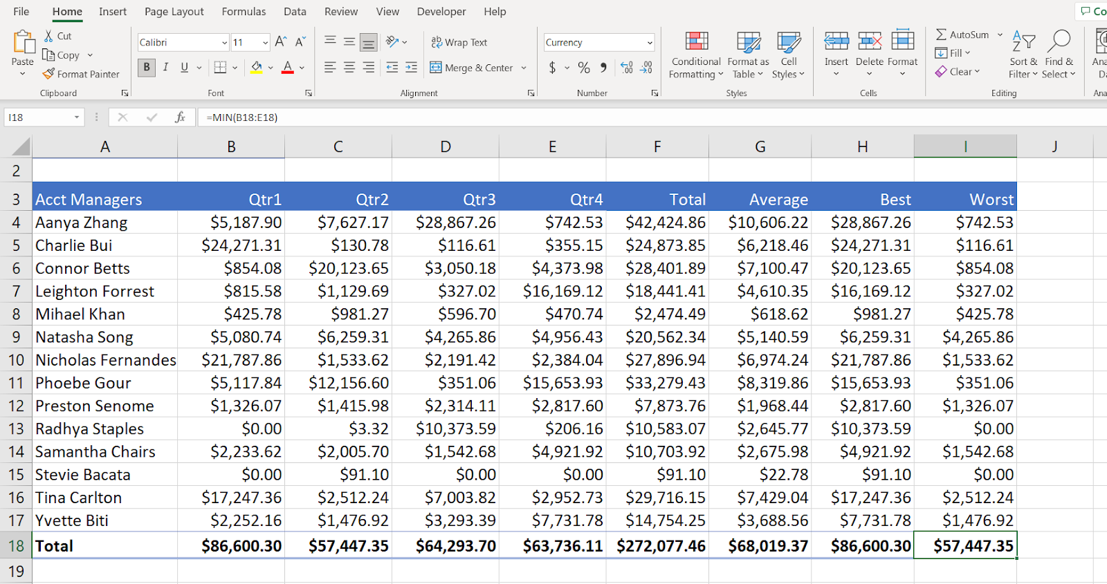
Now, after entering the function, we will press enter and get the result. 

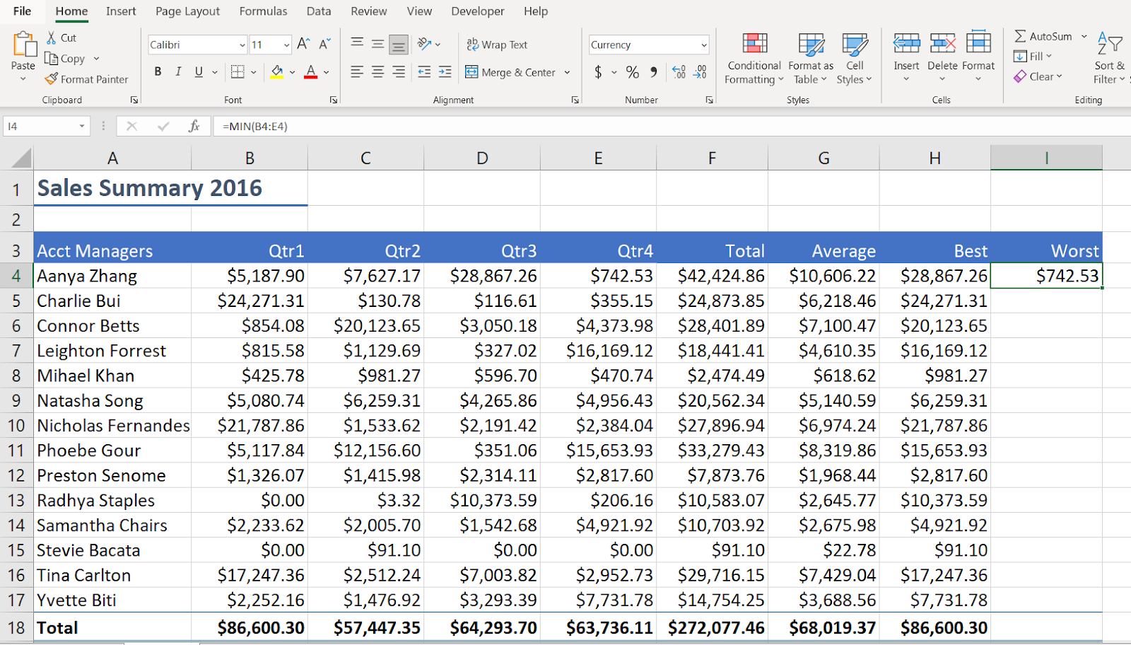
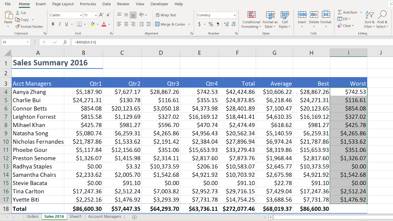
Now, if we want to know the lowest number for all the managers, use the fill handle, and we will get the lowest number for all the managers. 

Moreover, if we want to know the lowest total number among the four quarters, we can use the min function again. 

Put the formula where you want to see the number and press enter.

Excel will perform its magic and get you the lowest number. 

Now, let’s move to the next section.

Find the lowest number in Excel using the SMALL function

In this section, we will learn the easiest way to find the lowest number in Excel using the SMALL function. 

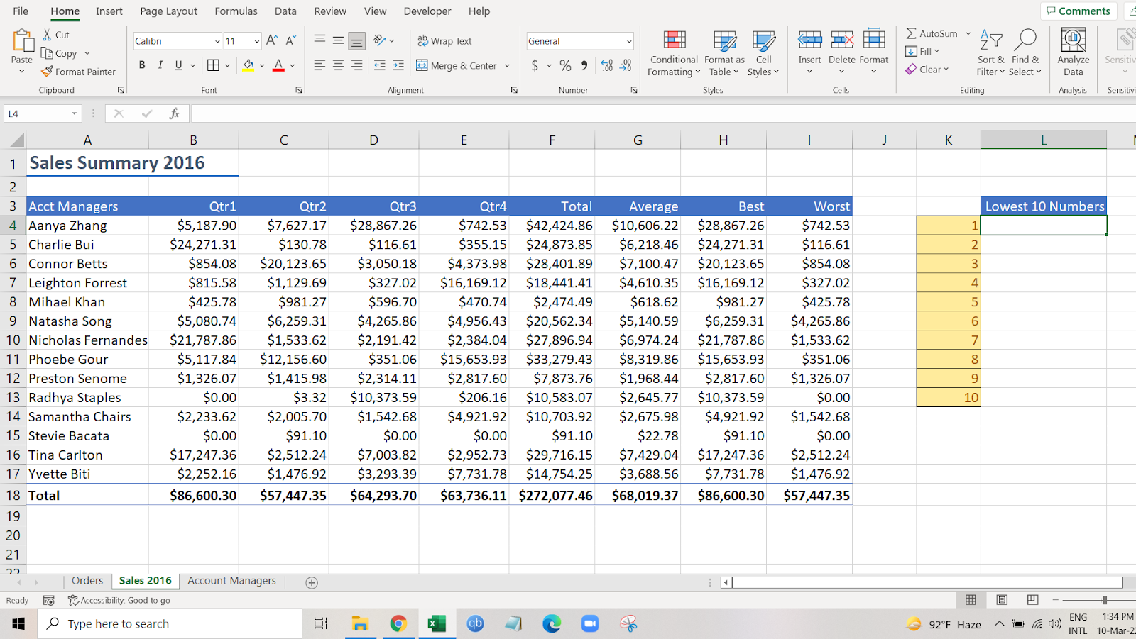
Here is our data. 

For example, we want to find the ten lowest amounts among all the managers’ quarters. 

To find out, we can use the SMALL function. 

So, 

Now, you are going to do magic with your formula, which is,

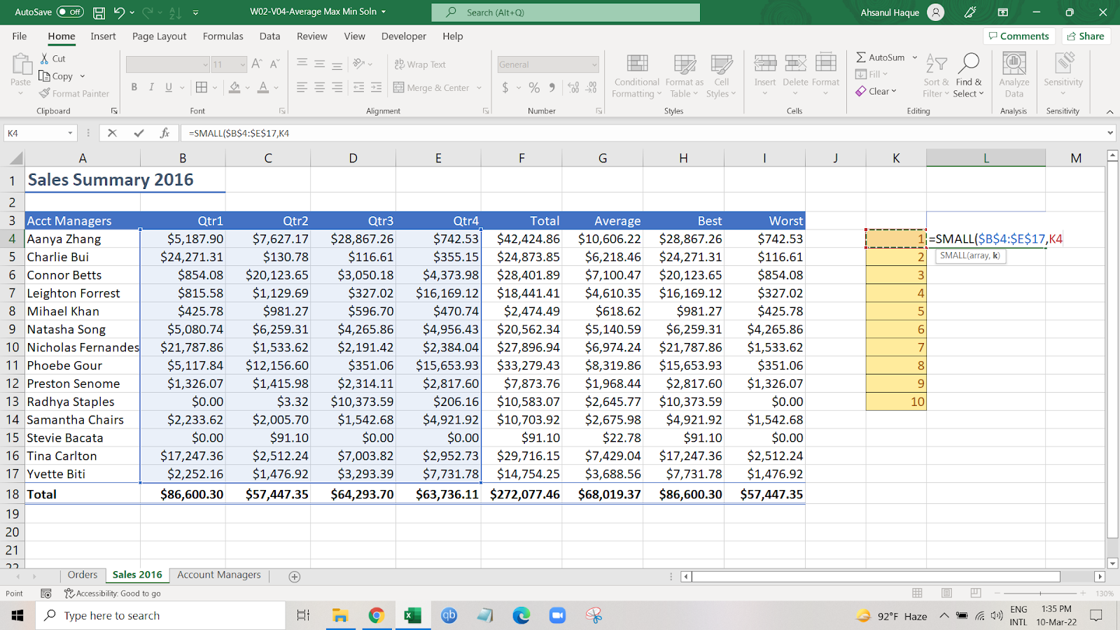
=SMALL($B$4:$E$17,K4)

=SMAAL(Array,k)

Explanation: 

• We selected the “Array” section from quarter one to quarter four data to determine the lowest 10 numbers among all the managers.
• We pressed “F4” to make the cell referencing absolute. We will talk about cell referencing in another article.
• We selected “K4” in k because we wanted to know the lowest number.
• And the other “K”s will find out which is the second smallest or third.

Learn More: F4 is not working in Excel

So, after entering the formula and pressing Enter, the result will look like this. 

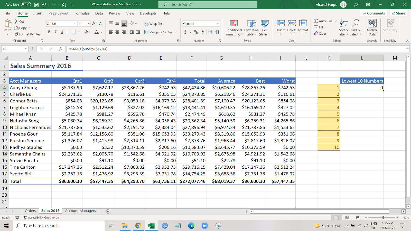
This shows 0 because it is the lowest number. 

Now, as we use the fill handle, it will show all the other lowest numbers. 

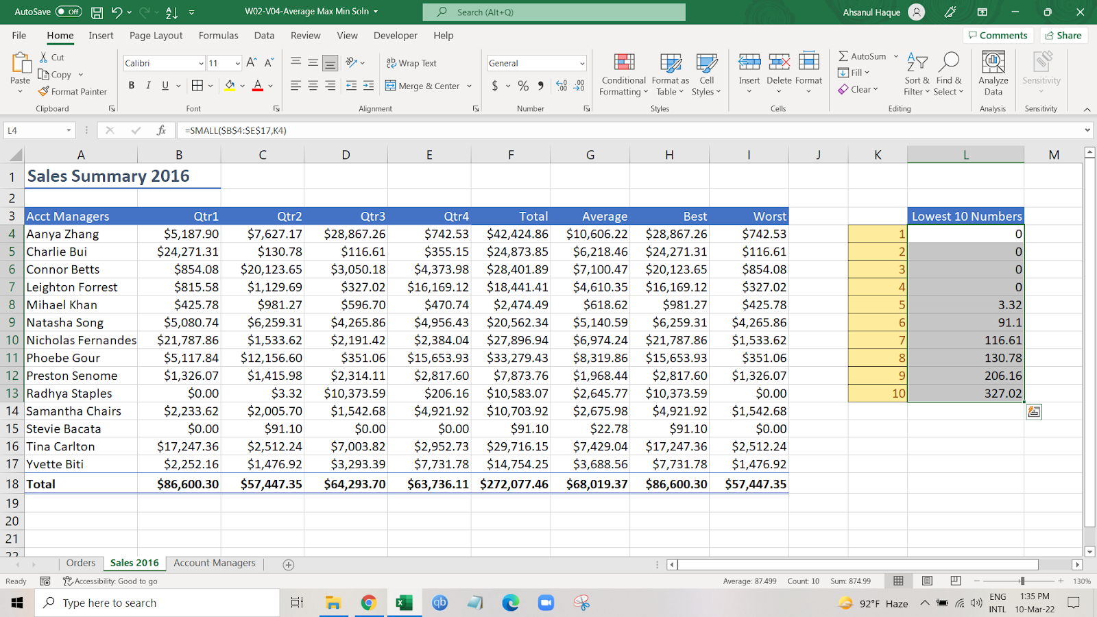
As we can see, it is showing all the other nine lowest numbers. 

In the formula, the tenth lowest shows 327.02 because we filled the “K” in the formula as 10 and selected K12. 

Another thing is, if we want to see the five lowest values in one cell, we can show this, too. 

For this, we won’t be needing the 1 to 10 list in the cell. 

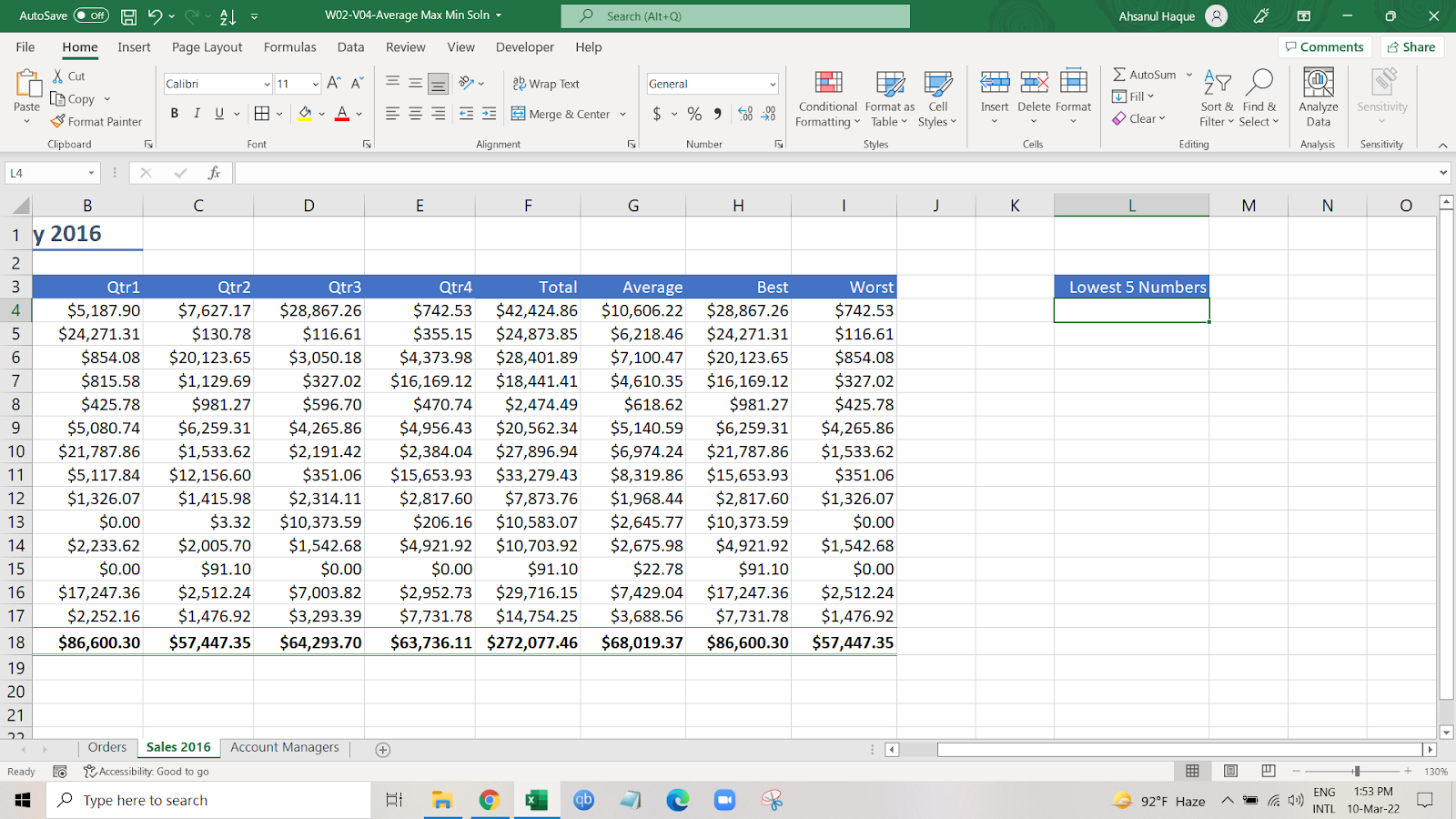
So now, we are going to put a formula. 

=CONCAT(SMALL($B$4:$E$17,1),”,”,SMALL($B$4:$E$17,2),”,”,SMALL($B$4:$E$17,3),”,”,SMALL($B$4:$E$17,4),”,”,SMALL($B$4:$E$17,5))

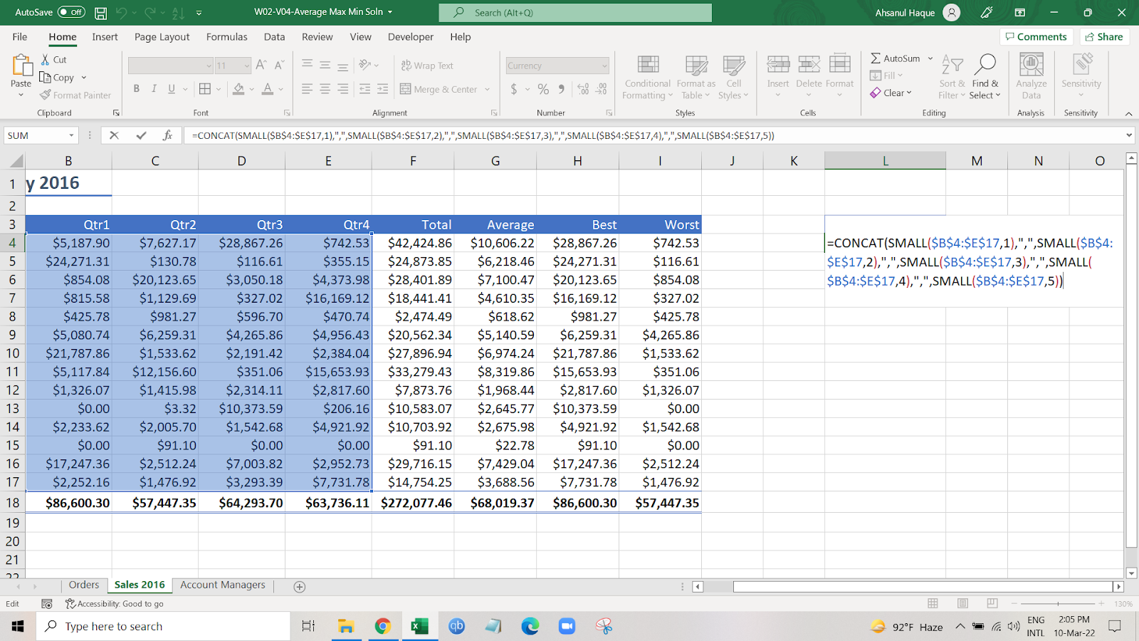
As we can see, this is a bit complicated and not advised to be used unless it is necessary. 

A little bit of explanation, 

• We found the first lowest number, and then used the “CONCAT” function to join the second lowest value with a comma.
• We repeated the whole process.

So that now we have seen 2 different approaches, we can move to another simple method.

Find the lowest number in Excel with conditional formatting

We can find the lowest numbers with conditional formatting if we just need a little summary of the data.

This method is only suggested to use if you need just an overview. 

So, step 1: Select the data. 

Step 2: go to your “Home” tab, click on the “Conditional formatting” , select “Top/Bottom rules” and then select “Bottom 10 items”.

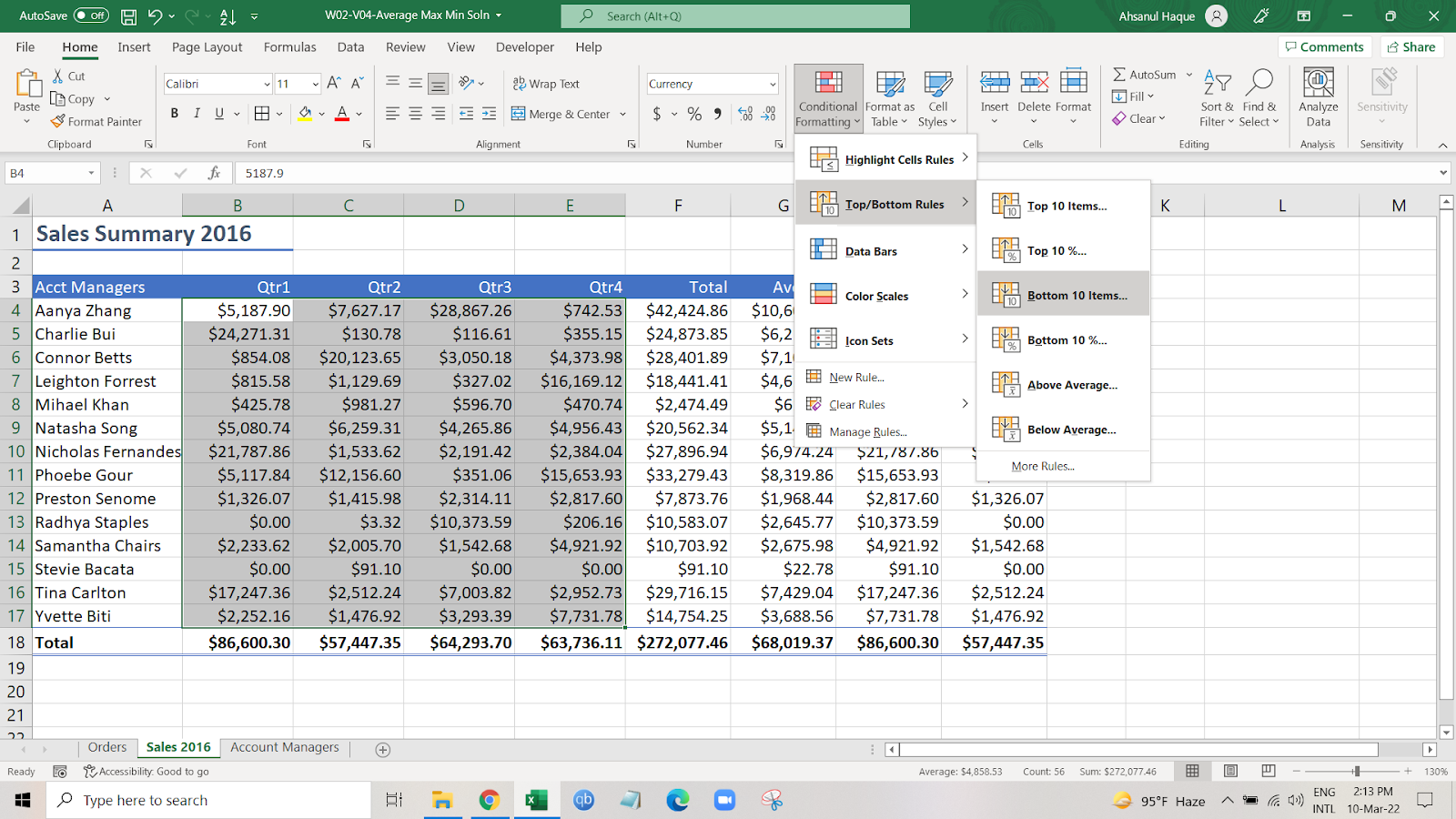
After clicking the bottom 10 items, it will show you this. 

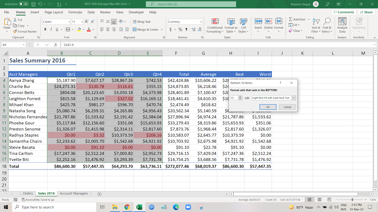
You can also change the item numbers.

For example, I just want to see the lowest 5 values. I will just change it to 5. 

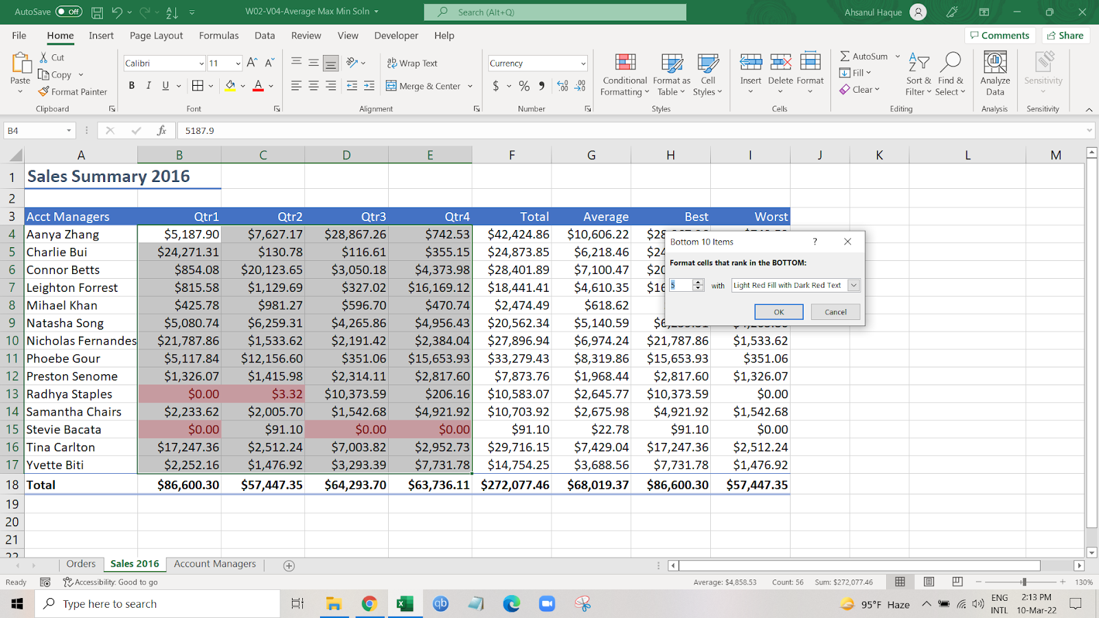
And it will show me the lowest 5 values. 

Find the lowest number in Excel using INDEX, MATCH, and MIN Function

We can also find the lowest value using INDEX, MATCH, And MIN Functions. This process is a bit complicated.

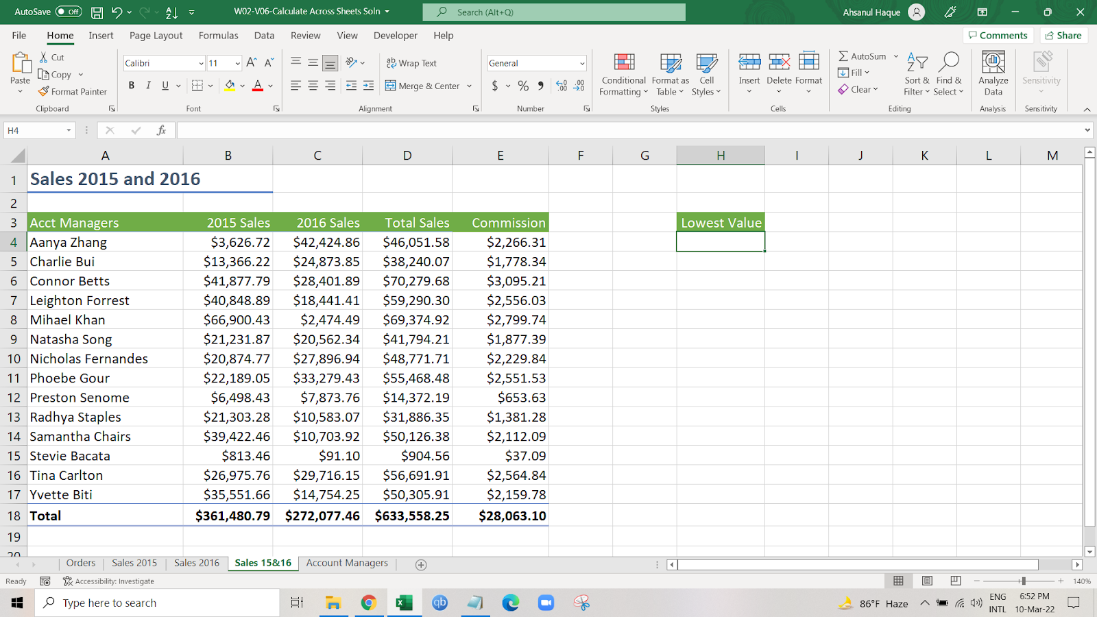
We have our data. We want to find the lowest number from any column without changing the whole function occasionally. To do that, we need lookup functions with dynamic functionality. 

So, here comes the INDEX and MATCH functions with the MIN function.

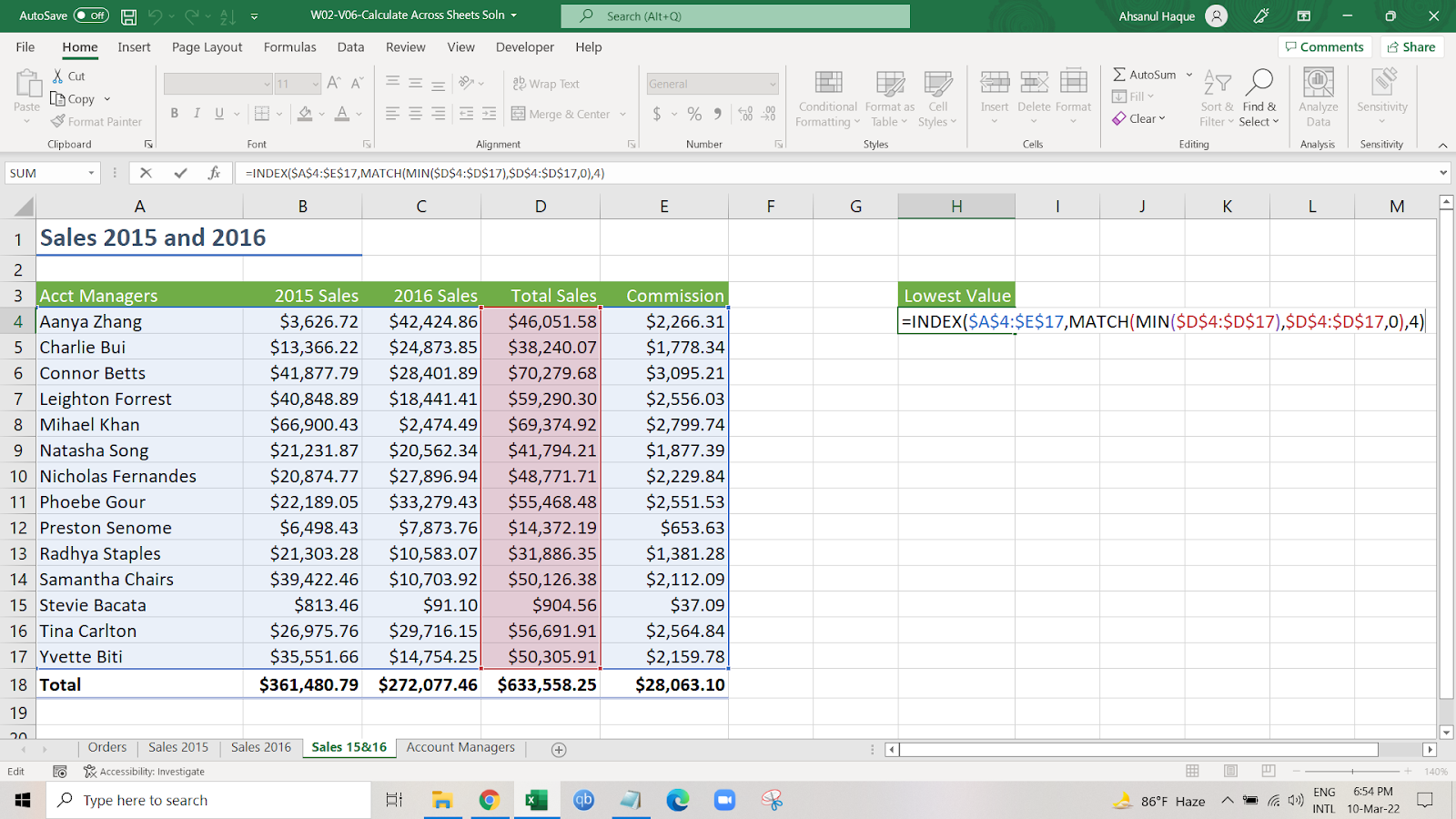
So, we are going to put the formula. 

=INDEX($A$4:$E$17,MATCH(MIN($D$4:$D$17),$D$4:$D$17,0),4)

Explanation: 

=INDEX (array, row_num, [col_num], [area_num])

=MATCH(lookup_value, lookup_array, [match_type])

• In the first part of the formula, the array was assigned to the whole data table because we wanted to occasionally find the lowest value from different columns or rows. 
• Then we combined it with the MATCH function, where we can assign the lookup value to find the lowest value with the MIN function, which will work to find the row number
• Then, we choose a specific column for the MATCH function array. You can choose any column for this array, whichever contains the numbers. 
• Then, you need to choose the same column as you chose before for the lookup array for the MATCH function as you have chosen for the MIN function.
• Then you want to find the exact match as match type, so type 0.
• The MATCH function’s purpose is to find the lowest value from any row. 
• The last part is from which column you want to see your lowest number. We typed 4 because we wanted to see the lowest number from the fourth column from the selected array as an INDEX function. This will work to find the column number.
• Then we press enter. 

Result:

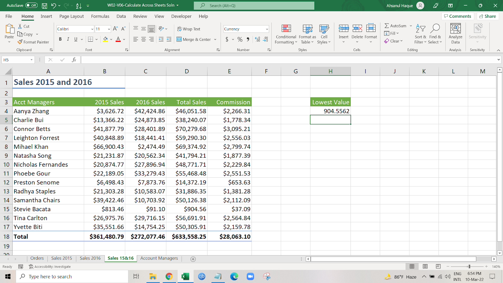
As we can see, it is showing the lowest number from the fourth column.

We can also easily show the lowest value from different columns.

 If we insert 2 in the col_num,  it will show the lowest number from the 2015 sales. 

Can we find out who has the lowest number among those account managers?

 Sure, we can just change the col_num to 1, and let’s see what happens. 

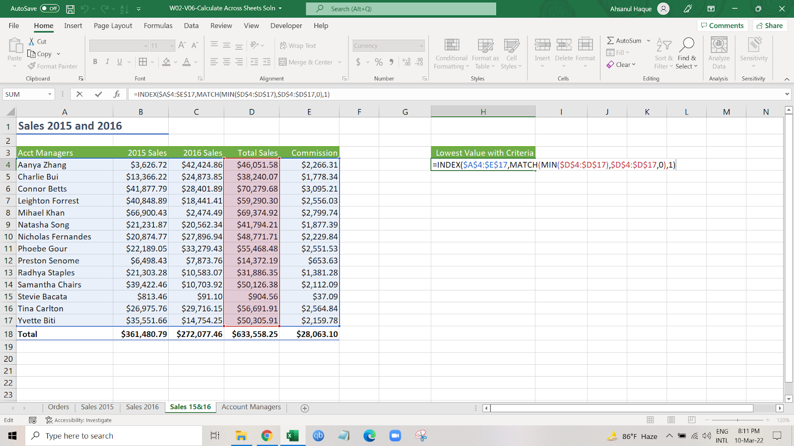
Press enter.

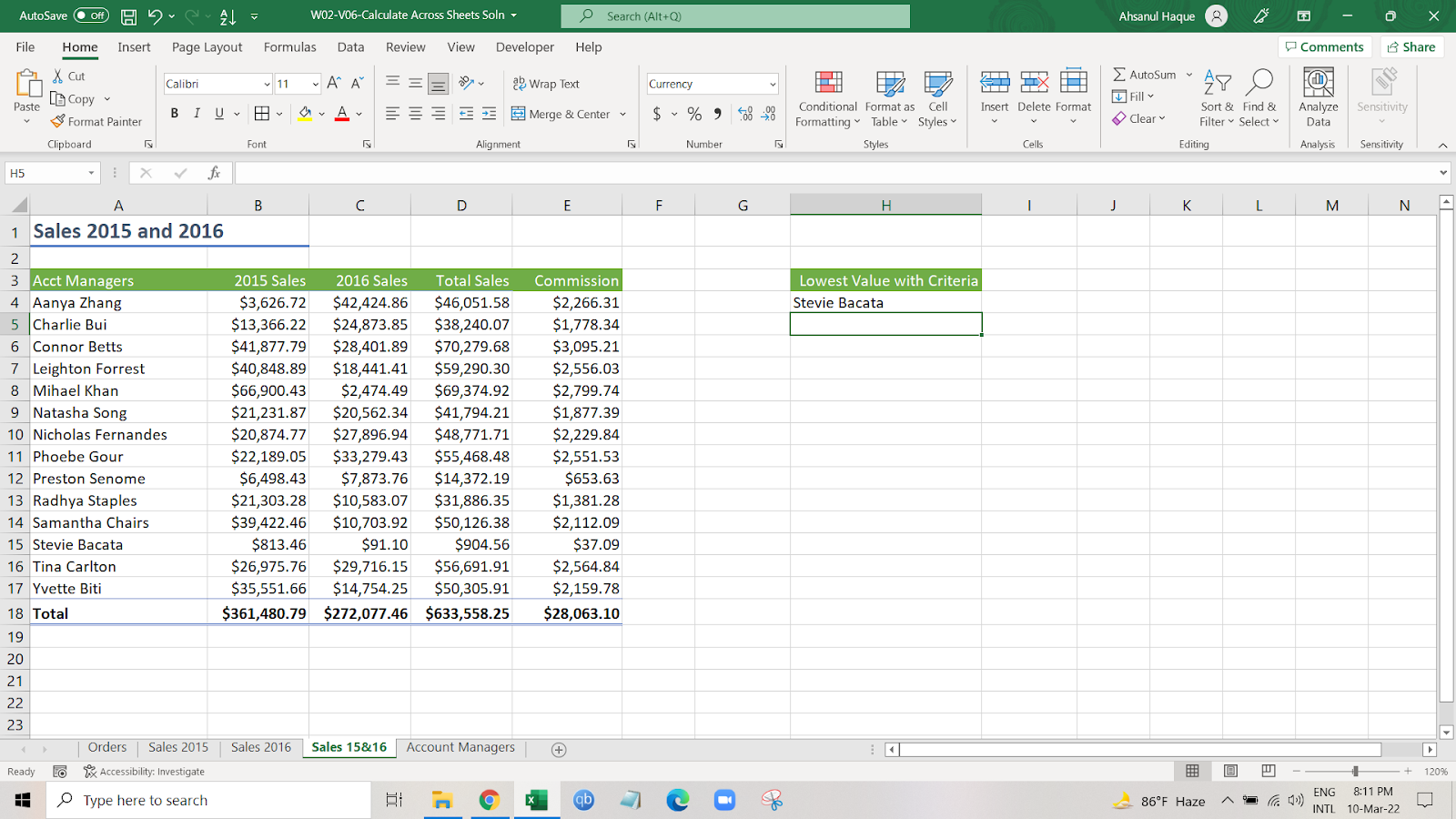
If we cross-reference the data, we can see that Stevie Bacata has the lowest number. 

Now that we have learned how to find the lowest number in Excel using the INDEX, MATCH, and MIN functions, let’s move to the following method. 

Find the lowest number in Excel With Criteria

In this section, we will learn how to find the lowest number using a simple function, MINIFS. We can find the lowest number with single or multiple criteria.

Find The Lowest Number In Excel Using the MINIFS Function with Single Criteria

Let’s look at our data first. 

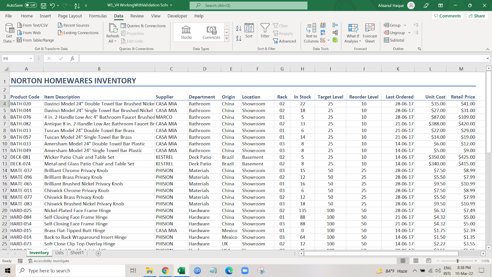
Now, we have a company’s inventory data. 

We want to find the lowest number in stock but with criteria. What criteria? We want to see if we are running short in “Showroom” or “Basement.” And if we are, by how much? Or what is the lowest number? 

So, first, we want to see if we are running low on the “Showroom” segment. 

Let’s insert the formula first. 

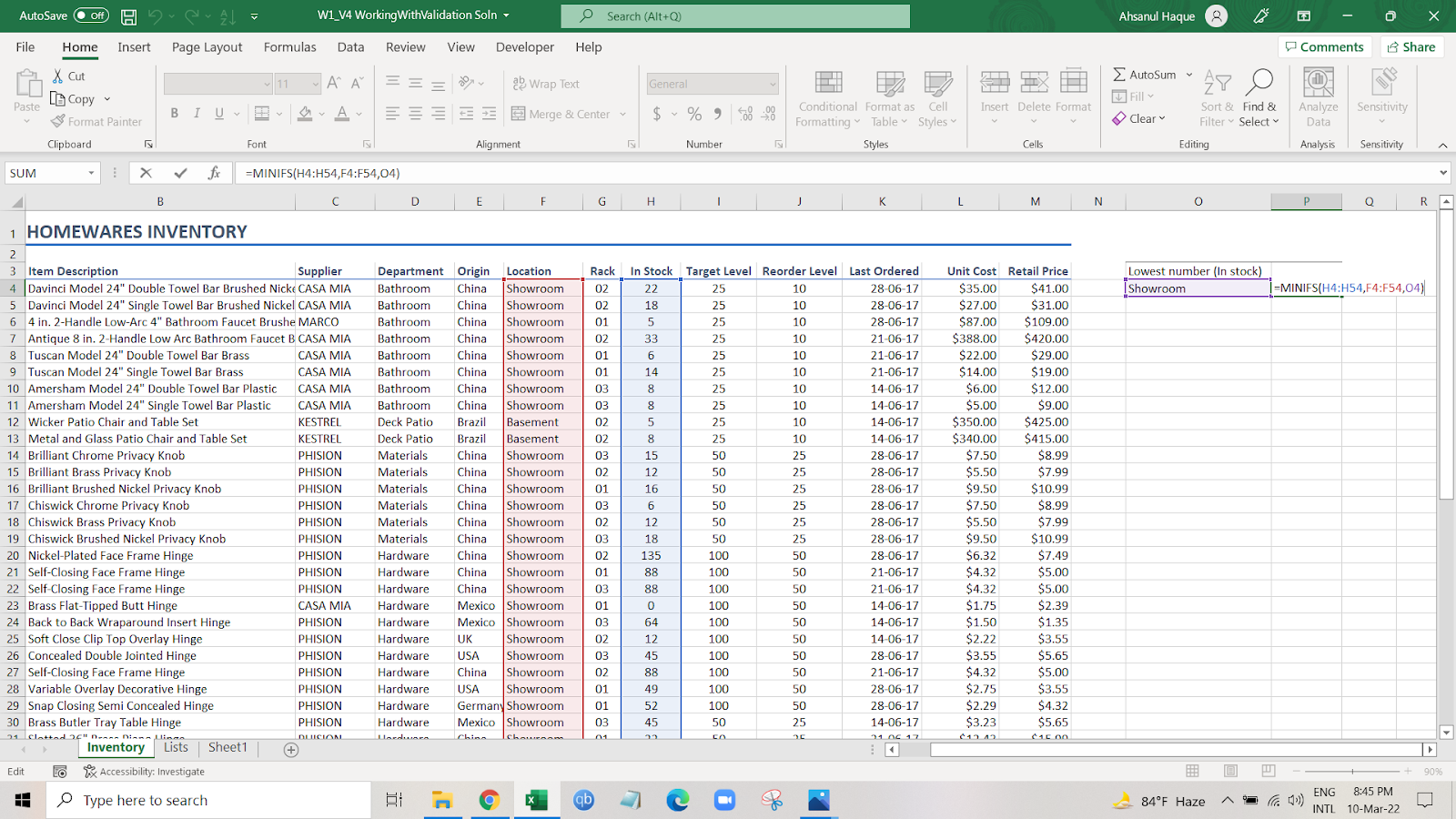
=MINIFS(H4:H54,F4:F54,O4)

Let’s see the formula with the arguments.

=MINIFS (min_range, range1, criteria1, [range2], [criteria2], …)

Here, 

• First, the min range refers to the column from where we want to retrieve the lowest numbers.  Which is in this from the “In stock” Column or H4 to H54
• Then, the second argument is what the criteria range is. In our case, this is the “Location” column where there are two different categories: showroom or basement or F4 to F54.
• The third argument is for which segment we want to find the number: Showroom. 

Now that we have inserted the formula. Press enter, and we can look at the result.

As we can see, in the showroom, the lowest number is 0. So that means we need to fill in the stock as quickly as possible. 

But can we find the lowest number for the “Basement” segment as well? Sure, we can.

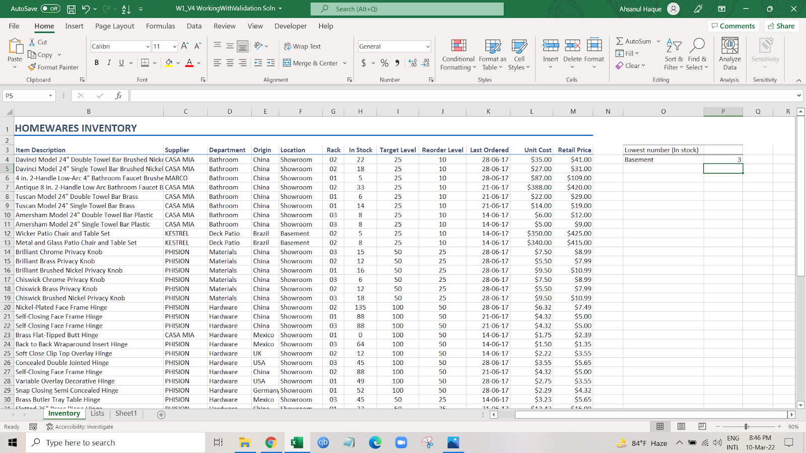
Just change the argument to Basement, and we are good to go. In this case, the result is 3, which means we are short in stock too for the “basement” segment. 

But what if you want to find the lowest number with multiple criteria? 

Let’s see how we can do that. 

Find The Lowest Number In Excel Using the MINIFS Function with Multiple Criteria

So, we want to find the lowest number with two criteria. 

One is the Basement, and the other is material. 

So, we want to find the lowest number for these two criteria. 

So, we are going to insert the formula now. 

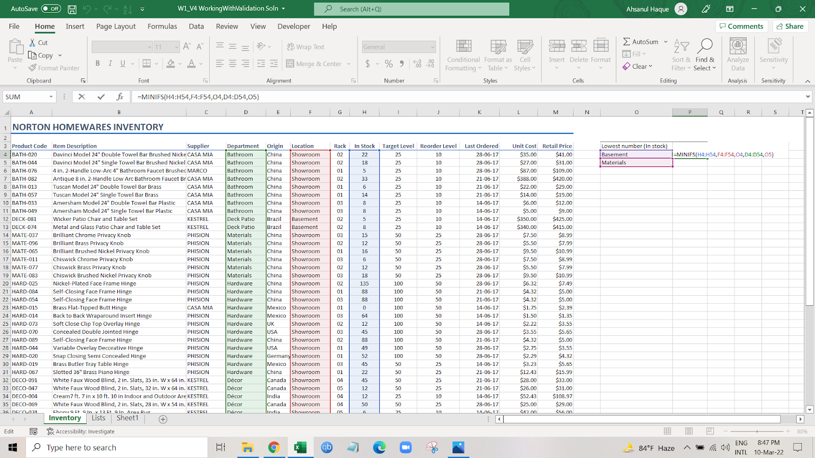
=MINIFS(H4:H54,F4:F54,O4,D4:D54,O5)

Here we added another criterion which is from the “department” section. There are 6 different segments, and we want to know the lowest number for “Materials”. So, we inserted that column as the 2nd criterion as augment and “Materials” as the 2nd criterion.

So, enter the formula and press enter.

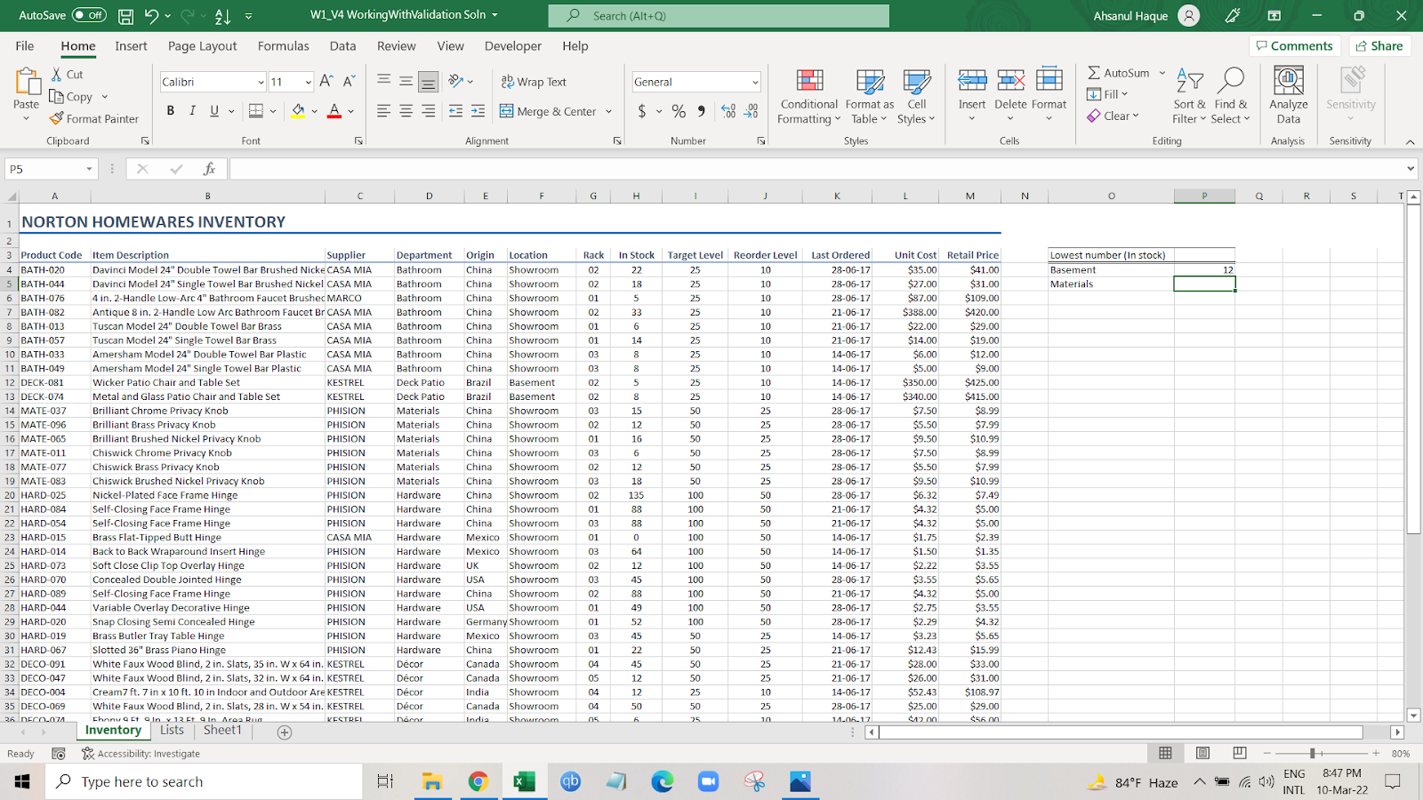
As we can see, excel is showing us the lowest number with two different criteria which is 12.

Can we find the lowest number for different criteria in the “department” column? 

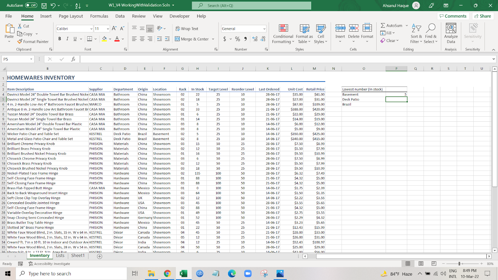
Let’s change the argument to “Deck Patio” and see what happens. 

As we can see, the lowest number changed from 12 to 5.

Can we increase the criteria? Yes, we can. 

Let’s see the data with 3 criteria. 

We want to see the data with the “country” or “origin” column. 

Let’s insert the formula. 

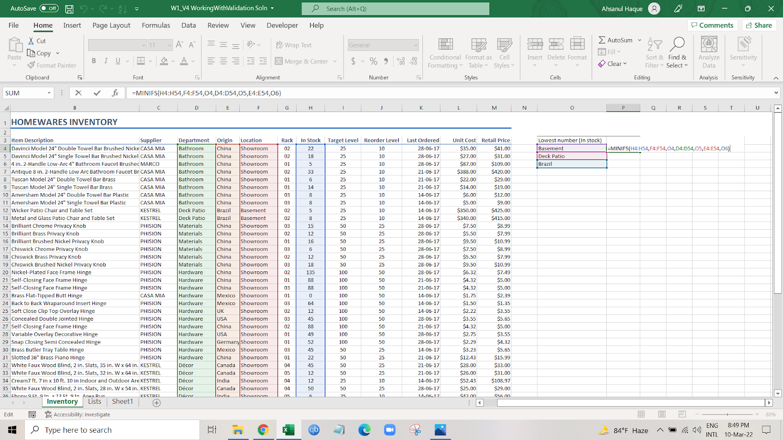
=MINIFS(H4:H54,F4:F54,O4,D4:D54,O5,E4:E54,O6)

So, this time we added another criteria range and other criteria for origin. Which is Brazil in this case. 

And if we press enter, we can see the result.

As we can see, it is showing the result. 

We can add as many criteria as we want.

This formula tremendously helps us to find the lowest numbers with different criteria.

We can find the lowest value using different methods. These are;

• Find The Lowest Number In Excel Using MIN & IF Functions with Single Criteria
• Find The Lowest Number In Excel Using MIN & IF Functions with Multiple Criteria
• Find The Lowest Number In Excel Using the SMALL IF Function with Single Criteria
• Find The Lowest Number In Excel Using the SMALL IF Function with Multiple Criteria (AND, OR method)
• Find The Lowest Number In Excel Using the AGGREGATE Function

This method uses array formulas, which is an advanced formula technique. We will learn about this in another article.