How to Change Chart Colors in Excel [3 Easy Ways]

To improve the chart’s overall aesthetics, sometimes we need to change the graph’s colors. And, in the new version of excel, there are more efficient ways now.

Here, I will walk you through how to change chart colors in Excel in 3 easy ways.  The ways are from the chart design ribbon and page layout ribbon.

Let’s discuss them in detail.

3 Ways to Change Chart Colors in Excel

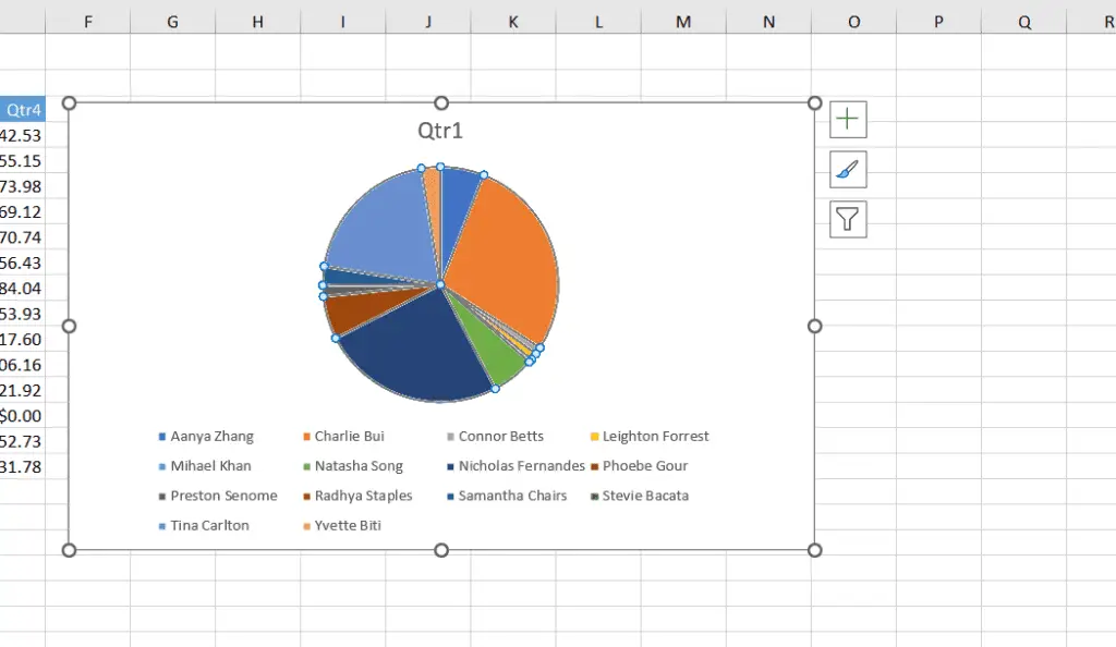
Here is a real-life example. We have a pie chart where you can see names and pieces assigned to each slice.

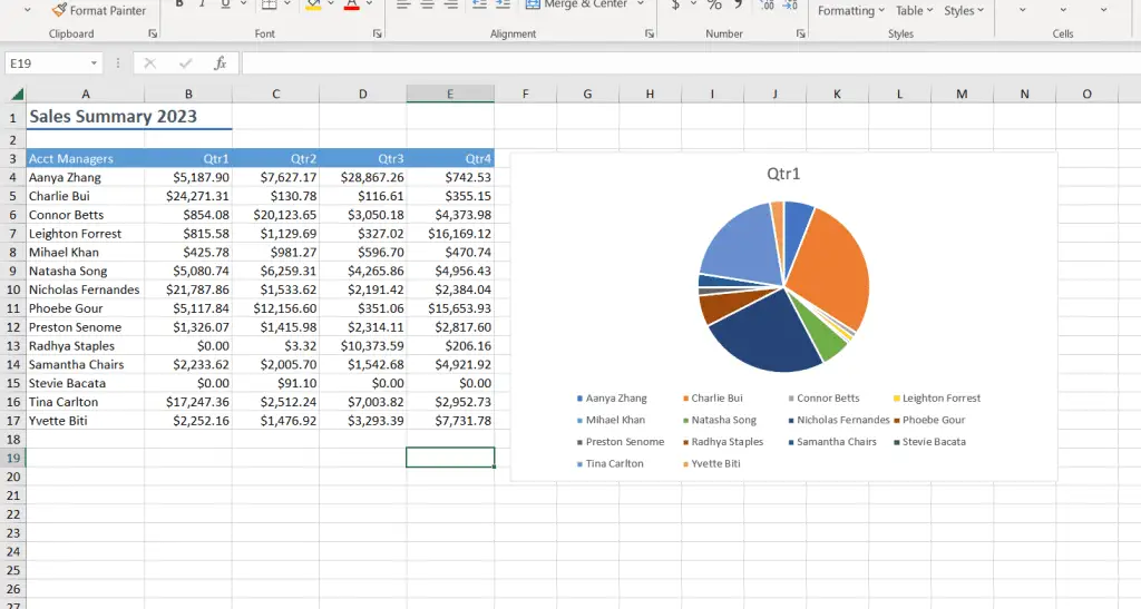
You can change the entire look of this chart just by changing the style or color. Let’s look at our first option.

Way #1: From “Chart Design” Ribbon

First, select the chart that you want to change color. Ensure that the chart border is selected, not the chart itself. Two new ribbons will pop up: Chart design and format.

Click on the Chart Design ribbon. There you will see many options, such as change chart type, move chart option, quick layout, add chart elements, chart styles, and the option we are looking for, change colors. 

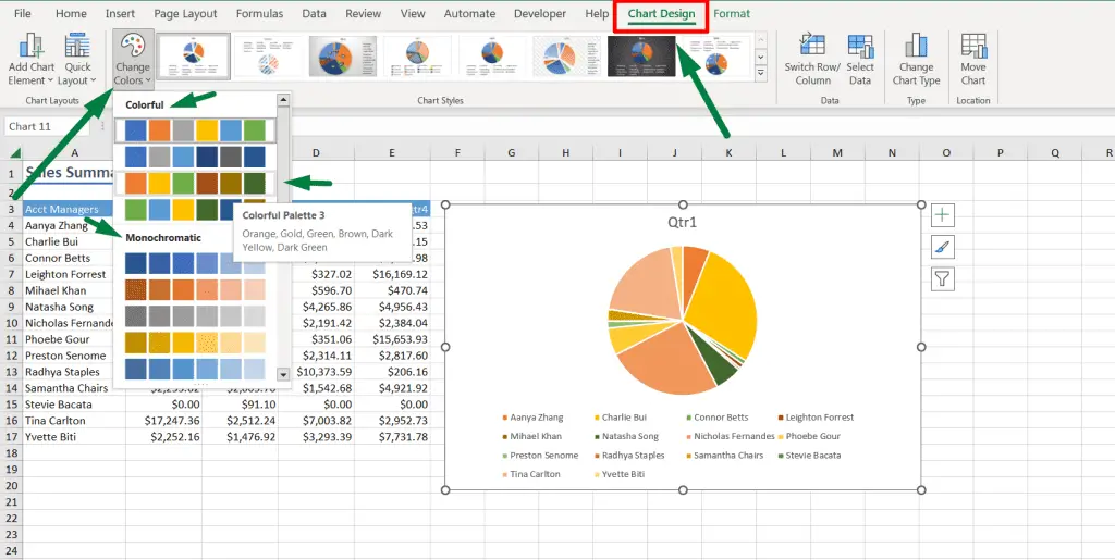
Click on the change colors drop-down option, and you will see two sections, colorful and monochromatic. 

Select any color section you prefer.

Or, you can use a keyboard shortcut. After selecting the graph, press Alt + JC + H, which will take you directly to the change colors option, and then you can choose as you prefer.

Way #2: From “Page Layout” Ribbon > “Colors” Option

Another option is from the page layout ribbon. Go to that ribbon. You will also find many options, such as the gridlines show or hide option, headings option, print titles, print areas, margins, orientations, etc.

But we don’t need these. We need the “Color” option in the theme section.

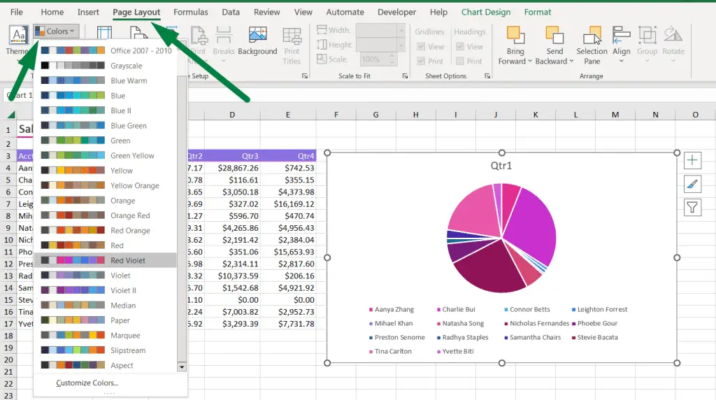
Click on the drop-down menu in the colors options; you will find tons of options, and you can customize colors from there. 

Or use this shortcut after selecting the chart: Alt + P + TC. It will take you directly to the color option in the page layout ribbon.

Way #3: From “Page Layout” Ribbon > “Themes” Option

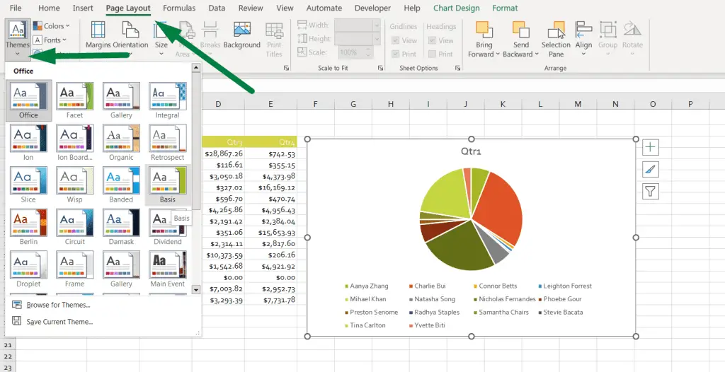
There is another option in the page layout ribbon, where you can change the color and overall looks, including fonts and other elements of the entire Excel sheet, which is the “Themes.”

You will find the “Themes” option in the themes section at the far left side of the page layout ribbon. 

Or you can press Alt + P + TH, which will open the themes drop-down menu, and from there, you can choose your preferred theme. Try out and see which one you like.

How to Change Individual Pie Chart Colors in Excel

Sometimes, you need to change just a slice of your pie chart. Here is how you can do that.

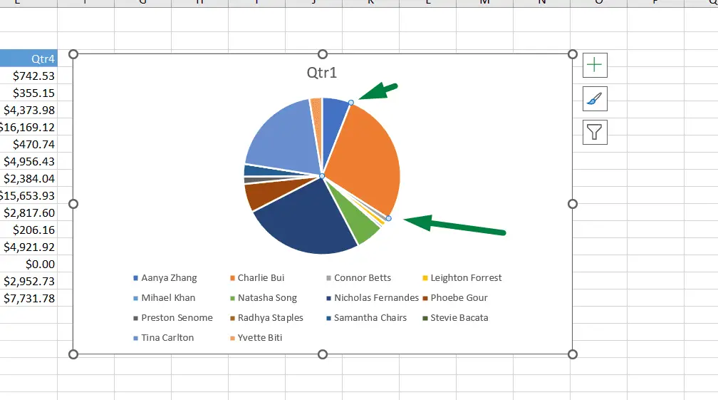
Click above the pie chart, and it will select all the slices. 

But, we want to change individual slice colors. So, again, click on the slice that you want to change. It will only select that slice.

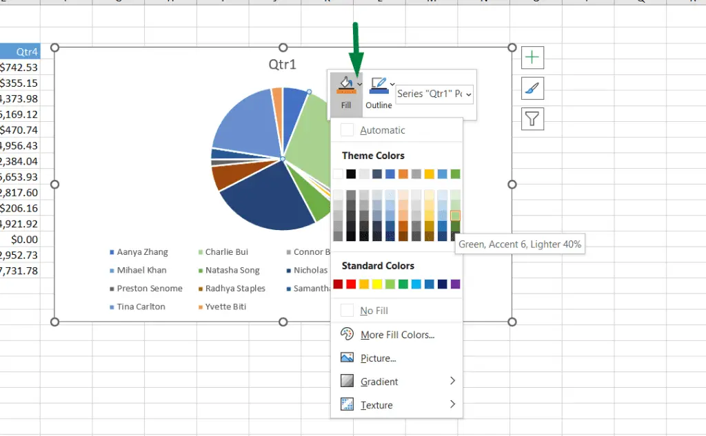
Then, you can change that slice’s color in two ways.

Way #1: RIght-click on the mouse, and it will show options. Click the drop-down menu of the “Fill” option, and it will display all the colors that are available for you to change.

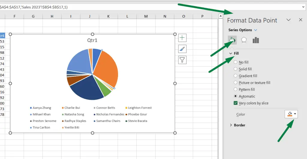
Way #2: After selecting that specific slice, double-click on that. It will open a sidebar named “Format Data Point,” and from there, click on “Fill and Line,” which is the first option. 

Go to the color option and change the color you prefer.

How to Change Background Color of Graph in Excel [3 Ways]

You can change the background of a chart. And you can do that in three ways.

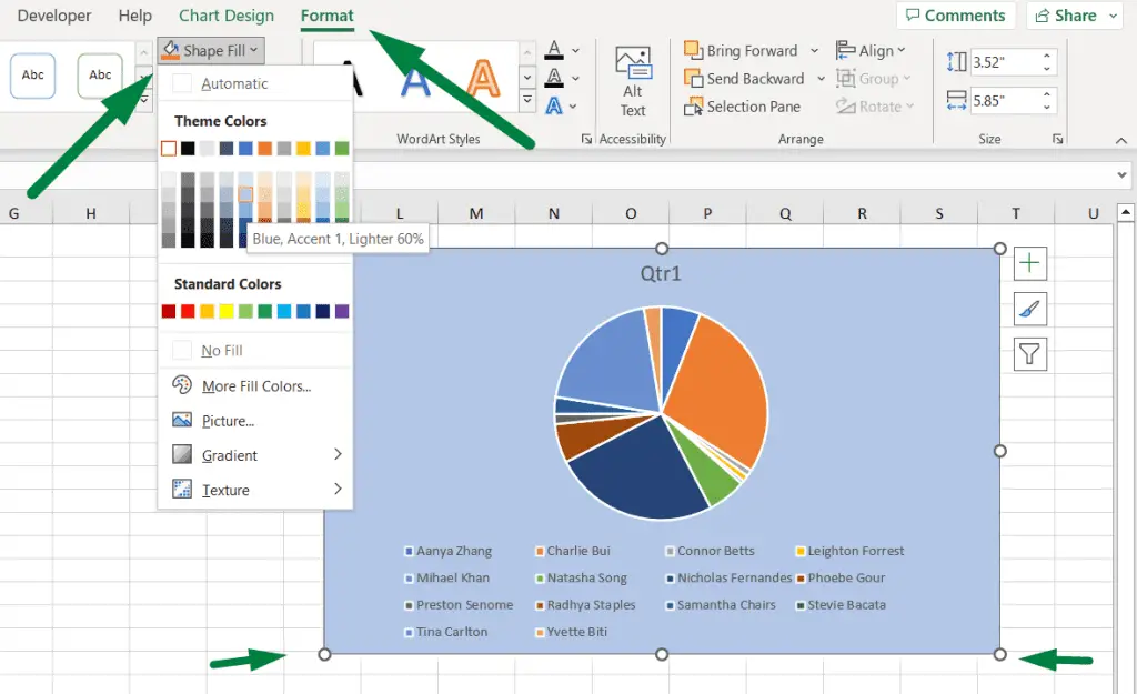
Way #1: From the Format Ribbon

1. Click on the chart area, not the chart itself. Ensure that the chart is selected and not the chart itself.
2. It will open two ribbons, chart design, and format. Go to the “Format” ribbon.
3. Click on the drop-down of the “Shape Fill” option.
4. Choose the preferred color you want for the background.

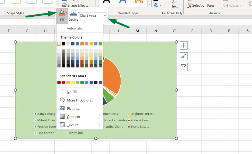
Way #2: Right-Click Option

You can also use the right-click option to change the chart’s background color.

1. Click on the chart area. You will see white colored round at the corners of the chart area.
2. Right-click on the mouse.
3. Click on the “Fill” option and choose the color.

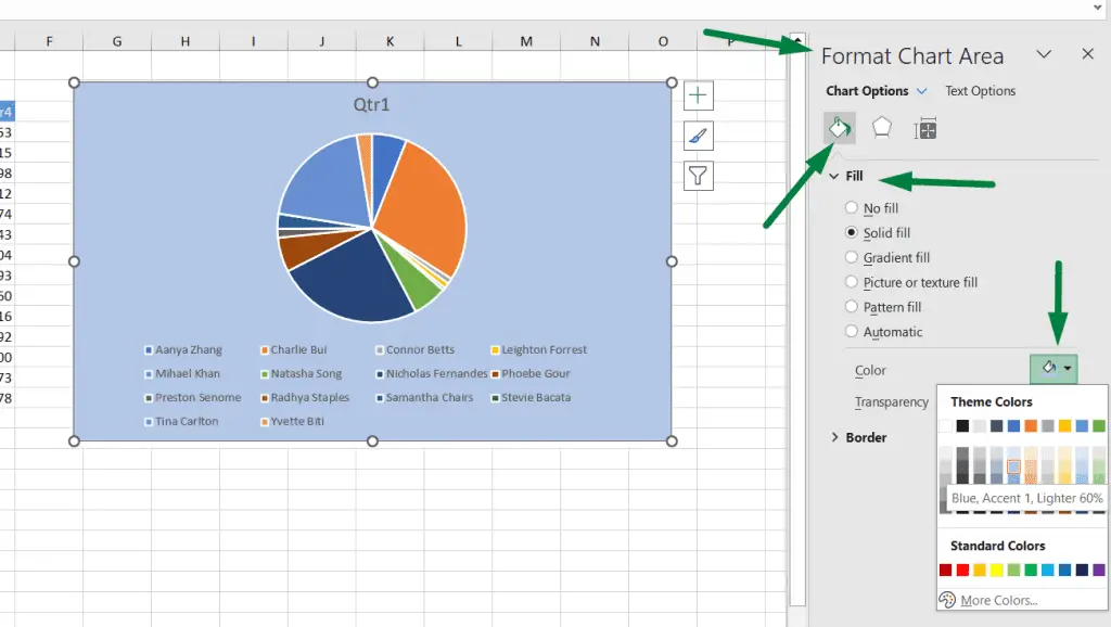
Way #3: From Format Chart Area Option

1. Double-click on the chart area.
2. It will open the “Format Chart Area” option on the right.
3. Go to the fill option.
4. Choose the color.

Summary

You can change chart colors in 3 ways.

1. Click on the chart > go to the chart design ribbon > click on the change colors and select the color.
2. Click on the chart > go to the page layout ribbon > click on the colors and select the color.
3. Click on the chart > go to the page layout ribbon > click on the themes and select any theme you prefer.

To change an individual bar or pie color in the graph;

1. Move your mouse cursor to that bar or slice of the pie chart > Right-click on the mouse > click on the fill option and choose your color.

To change the background of the chart;

1. Select the chart > Go to the format ribbon > Click on the shape fill and choose a color.
2. Select the chart > Right-click on the mouse > Select the fill option and change the color.
3. Double-click on the chart area > “Format Chart Area” option > Go to the fill option > Choose your preferred color.