How to Change A Chart Style in Excel (In 3 Clicks)

Visualizing tons of data using a chart or graph is a fantastic idea. But, when you create a chart in Excel, it gives you a default chart style. But, sometimes, you might need to change the style, so I’ll show you how to change a chart style in Excel.

But, in brief, select the Chart > press Alt + JC > Select the style.

I’ll show the process in detail with pictures. Let’s get into it!

What Is A Chart Style In Excel?

A chart style is an all-in-one solution for changing a graph’s overall look and feel, such as chart color, background, etc. 

Besides, it saves you the hassle of going through all the options of elements and everything that comes with formatting a graph.

Within a few clicks, you can change the overall look of a chart.

How To Change A Chart Style In Excel (Step-by-Step)

As I said, you can change the chart style within just 3 clicks. Let’s see how;

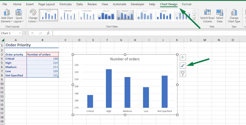
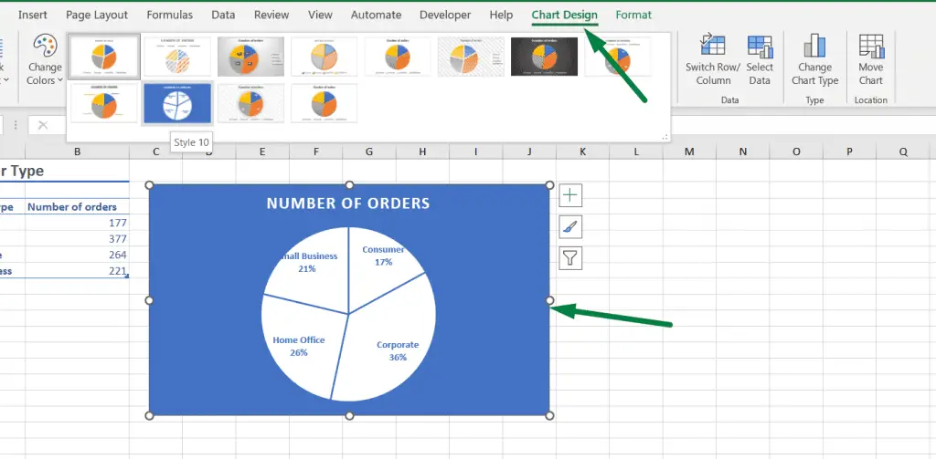
Click #1: Select the chart. It will open two new ribbons named “Chart Design”  and “ Format”  in the ribbon area.

Click #2: Then, click on “Chart Design,” and you will see a section named “Chart Styles.”

Click #3: You can choose any chart style you prefer. But there are more chart styles available.

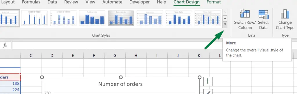
Click on the small drop-down option, as shown in the picture. It will display all the options or styles for that chart.

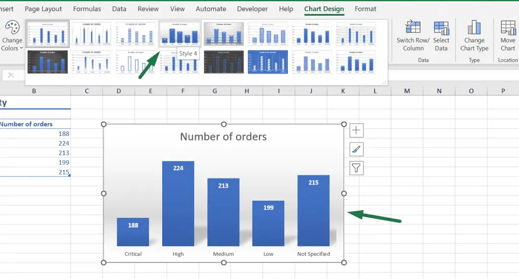
For example, I choose style 4, and Excel will show my chart like this.

Tip: You can also change the chart type from the chart design ribbon.

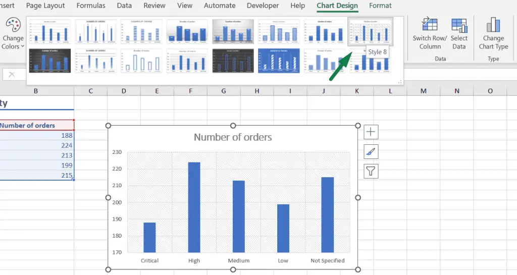
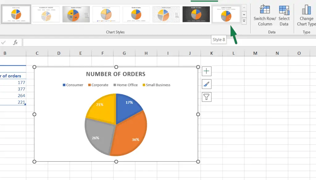
Another example: How to change the chart style to style 8 in Excel

Similarly, if you want to change the chart style to 8, click on the chart > go to the chart design ribbon > select “ Style 8” at the top right. 

How To Change Pie Chart Style In Excel

There is more! You can change the chart style for any chart you want.

For example, you can change the pie chart style similarly.

Select the pie chart > Go to the chart design ribbon > select your preferred style. 

For different charts, style 8 could be different. For example, when I change the style of my pie chart to style 8, the overall background, color, and looks are different.

Summary

So, here’s how we can change chart style in Excel within 3 clicks.

1. Click on the chart or graph.
2. Click on the “Chart Design” ribbon.
3. Click on your preferred chart style.

The Shortcut to go to the “Chart Design” ribbon: Alt + JC