How to Change Chart Type In Excel [In 2 Ways]

Sometimes, you might need to change the chart type for better readability and make it more understandable.

And that’s why you need to know how to change chart type in Excel.

First, click on the chart > It will open two new ribbons named “Chart Design” and “Format” in the ribbon area > Click on the “Chart Design” ribbon > Click on the “Change Chart Type” option, which will open a box > Choose your preferred chart type which you want to change. 

Or click on the chart and press the “Alt + JC + C” shortcut to open the “Change Chart Type” box. Then, select your preferred chart type.

There is another easier way. I’ll show you how to do this in detail in the following section and all the related options.

How to Change Chart Type In Excel (Easy Steps)

You can change the graph type in 2 ways. The first one is the traditional and the second way requires only two clicks.

Way #1: From the “Chart Design” ribbon.

Here are the steps on how do you change the chart type of an existing chart.

Step #1: Click on the Chart or Graph.

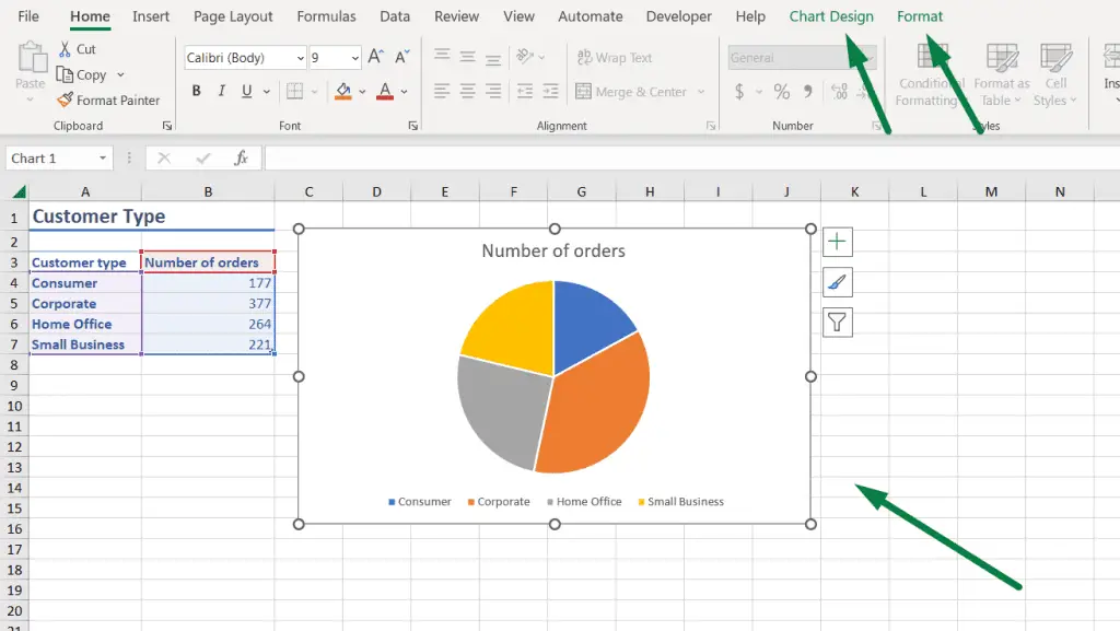
It will open two new ribbons. One is “Chart Design,” and the other is “Format.”

Step #2: Click on the “Chart Design” ribbon and select “Change Chart Type.”

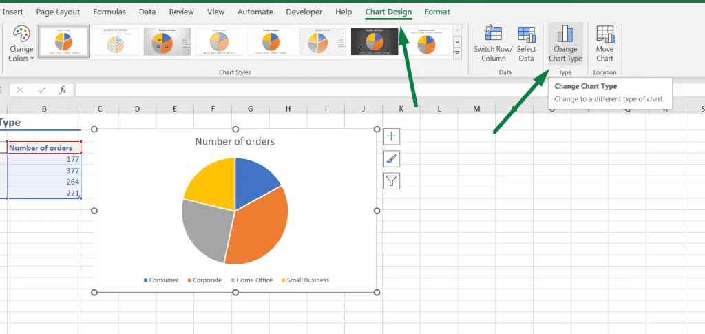
It will open a box named “Change Chart Type”

Note: You can also change chart styles from here.

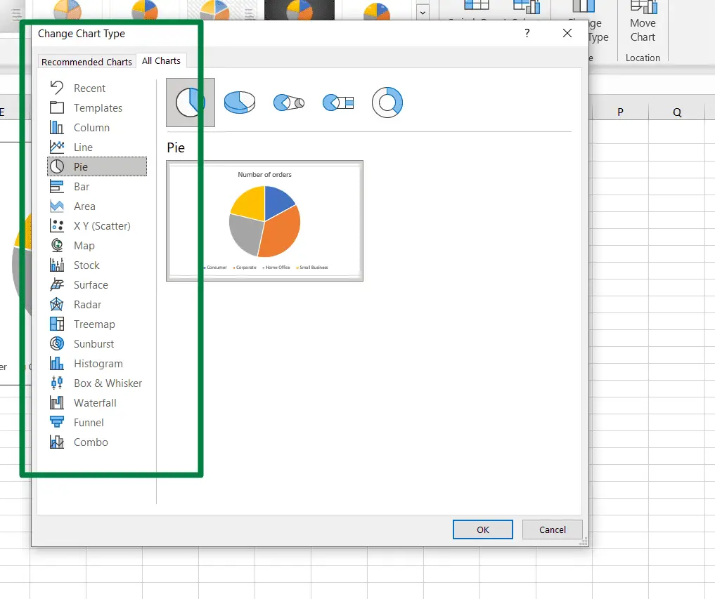
There, you will find all the chart types. You can choose any chart types you prefer. For example, you can change the type into a bar or column chart. And there are more options.

Example #1: How to change chart type to clustered column in Excel

Click on the “Column” option. You will have a “Clustered Column” option; click on that. 

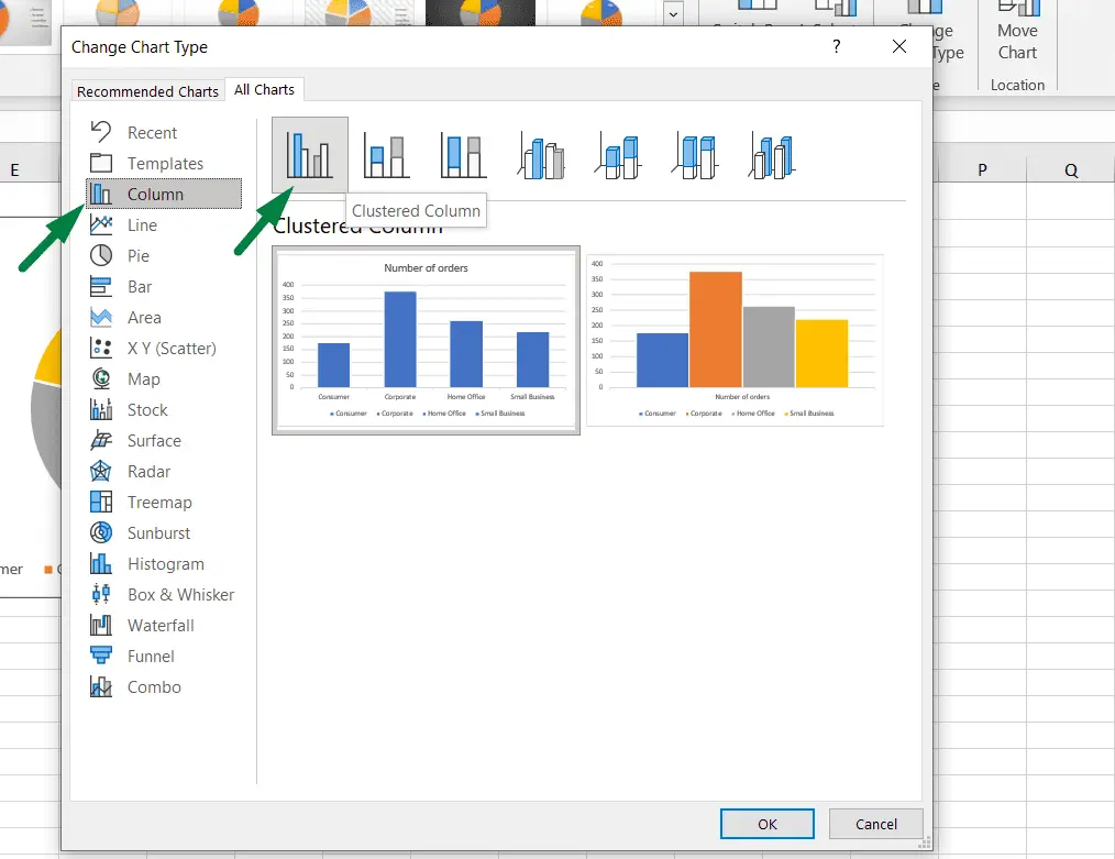
Besides, there are other options, such as 3-D clustered column, stacked column, and 3-D stacked column options.

Example #2: How to change the chart type to the first stacked bar option in Excel

Click on the “bar” option. The second option from the left is the stacked bar; click on that.

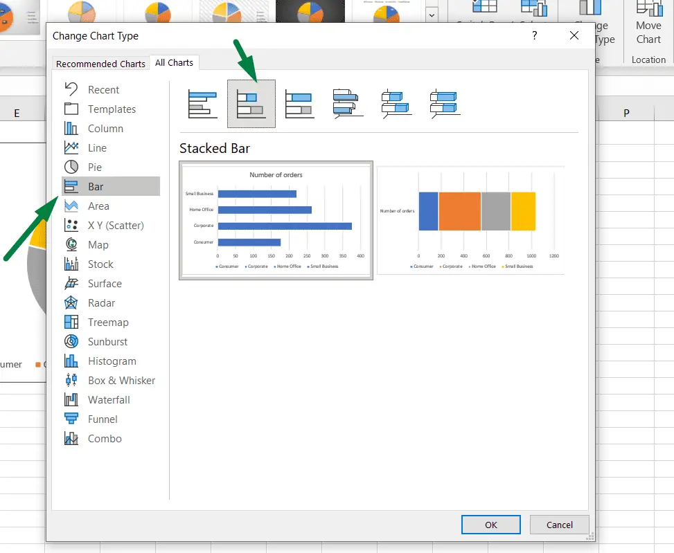
There are also clustered bar and 3-D stacked bar options in there.

Way #2: Right-click on the mouse.

First, move the mouse cursor above the graph and right-click on the mouse. It will open a list of options.

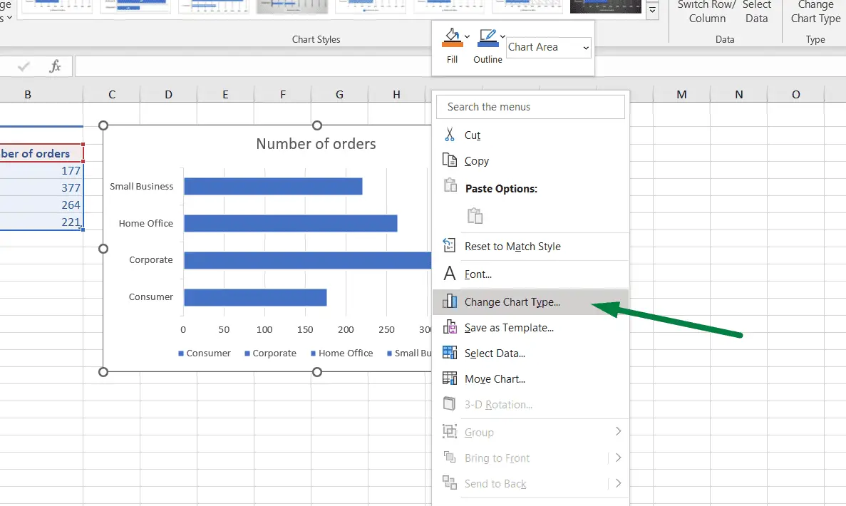
Click on the change chart type option to open the box where you can change the chart type.

Why Can’t I Change My Chart Style In Excel?

Sometimes, there might be trouble changing the chart style in Excel. When you click on the chart design or format ribbon, you might find that the ribbons are grayed out. It means that you can’t access the change chart type option.

There is no exact cause why you can’t change the chart style in excel.

But I tried to find some solutions, and here are they.

Way #1: Older version of the file.

One of the reasons could be the version of the Excel file you’re using. They may have been created in the 97-2003 version (*xls).

In that case, you must save the file in Excel Workbook (*.xlsx) format. Press “Ctrl + S” to the “Save As” tab and save the file.

Way #2: Copy all the sheets to a new workbook.

If you can’t find any reason or solution, select and copy all the sheets to another workbook. That might solve the issue. 

Summary

You can change the graph or chart type in Excel in 3 ways.

1. Select the chart > Click on the “Chart Design” ribbon > Select the “Change Chart Type” option > Choose the chart you prefer.
2. Select the graph or chart > Press Alt + JC + C > change the chart type.
3. Move the mouse cursor above the graph > right-click on the mouse > Select the “Change Chart Type” option.

If the chart design ribbon is grayed out or you can access the “Change chart type” option, then

• Either save the file from 97-2003 (*xls) version to Excel workbook (*xlsx) format.
• Or, copy all the sheets to a new workbook.