How to Make Graph Paper in Excel (7 Easy Steps)

There are several uses of graph paper. Whether you’re working in a statistical field, mathematics, or anything related to data, you might sometimes need to know how to make graph paper in Excel.

First, we need to format the row height and column width. Then, enable the print option, customize the margins and gridlines of that sheet, and you can even print the graph paper afterward.

Now, we will learn exactly how to do that step-by-step in detail. 

How to Make Graph Paper in Excel (Step-by-Step)

You can do much more, plotting graphs or data points using graph paper. Now, there are ways to draw graph paper in Excel.

After making the graph paper using Excel, you can print it at your convenience. Let’s dive into it.

Step 1: Select All the Cells/Whole Sheet

Our first sheet is to select the cells or the whole sheet. As we want to make graph paper, it would be convenient to select the entire sheet.

To select the entire sheet, click the ‘Triangle’ on the far left upper side. You will find that between column ‘A’ and row ‘1’, as shown in the screenshot. 

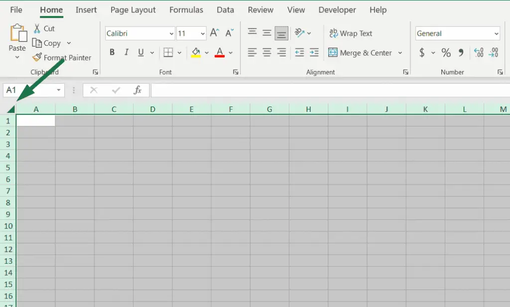
Select any blank cell, and press ‘Ctrl + A’ to select all the cells in that sheet. 

Step 2: Adjust ‘Row Height’ and ‘Column Width’ in Your Sheet

As we know, the row height and column width are different by default and are not square. 

The row height and column width of the cells is 15 and 8.43, respectively. And it looks like a rectangle. But we need to make it look square.

We can make the cells look square by changing the row height and column width.

Let’s do that!

In the ‘Home’ ribbon, click on the drop-down menu of the ‘Format’ option. Or press “Alt + H + O” to open the ‘Format’ tab.

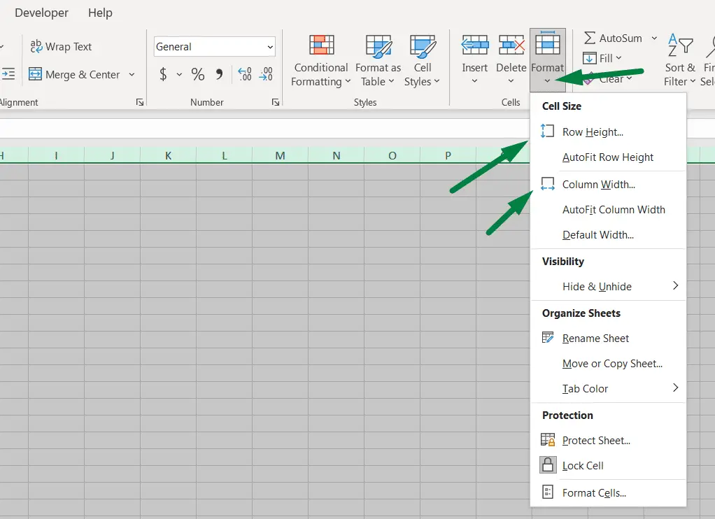
There you will find the ‘Row Height’ and ‘Column Width’ options.

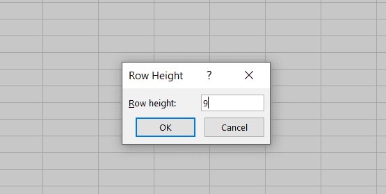
Click on the ‘Row Height’ option and insert ‘9’ (or 12). Then, click OK.

[Or you can use a shortcut to open the ‘Row Height’ option: Alt + H + O + H.]

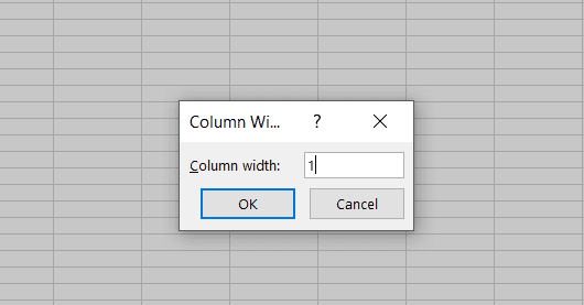
Again, Click on the ‘Column Width’ option. Insert ‘1’ (or 1.44). And click ok.

[Or you can use a shortcut to open the ‘Column Width’ option: Alt + H + O + W.]

Now that we completed our main part, which is making the sheet look like graph paper, we can move into our next section. 

We need to enable the print option to print the sheet with gridlines. Let’s see how to do that! 

Step 3: Enable or Tick Mark the Gridlines for Print

After making the sheet look like graph paper, we need to enable the print option for this sheet.

Go to the ‘Page Layout’ ribbon, then tick mark on the ‘Print’ option under the ‘Gridlines’ section. You will find this in the ‘Sheet Options’ section.

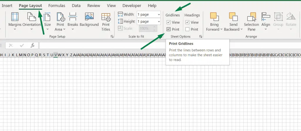
Or you can use a shortcut to enable the print gridlines option, ‘Ctrl + P + PG.’ It will print gridlines when you print the graph paper and any sheet.

Note: you can also show or view gridlines and hide them from this option.

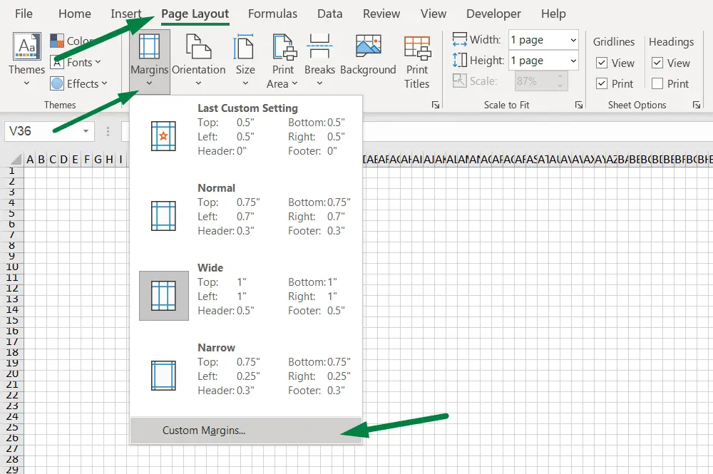
Step 4: Customize the Margins

Now, we need to customize the margins. Go to the ‘Page Layout’, click on the ‘Margins’ option, and select the ‘Custom Margins’ option. 

Or press ‘Alt + P + M + A’ to open the custom margins.

Then, set the top, right, bottom, and left margin at .5 and the header and footer at 0.

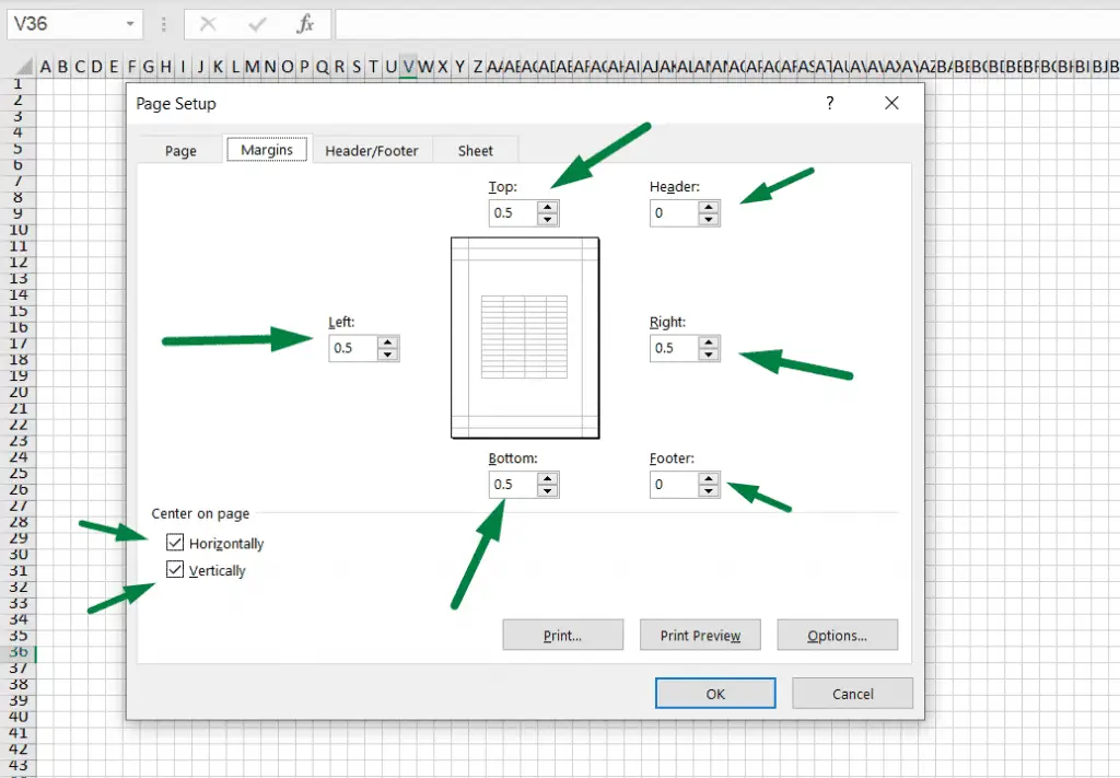
Then press ok. 

Step 5: Select the Paper Size

Now, we can select the paper size for the graph paper. Excel comes with various paper sizes, so choose one at your convenience.

I will select the ‘A4’ option for my graph paper. Go to the ‘Page Layout’ ribbon, and click on the ‘Size’ option under the ‘Page Setup’ Section.

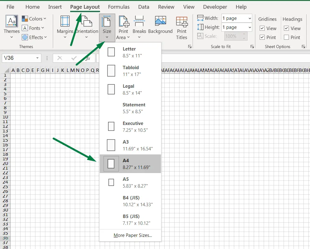
Select the paper size where you want to print your graph paper.

Step 6:  Select the Print Area

Now, we need to select the print area.

At the right-bottom corner, select the ‘Page Layout’ option and make the zoom button 40%.

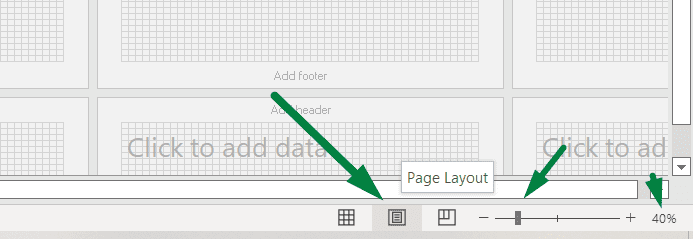
It will help you show the entire page, and then you can select the whole area which you want to print.

Select all the cell areas you want to print. And as we choose A4 size, the page will be shown at that size.

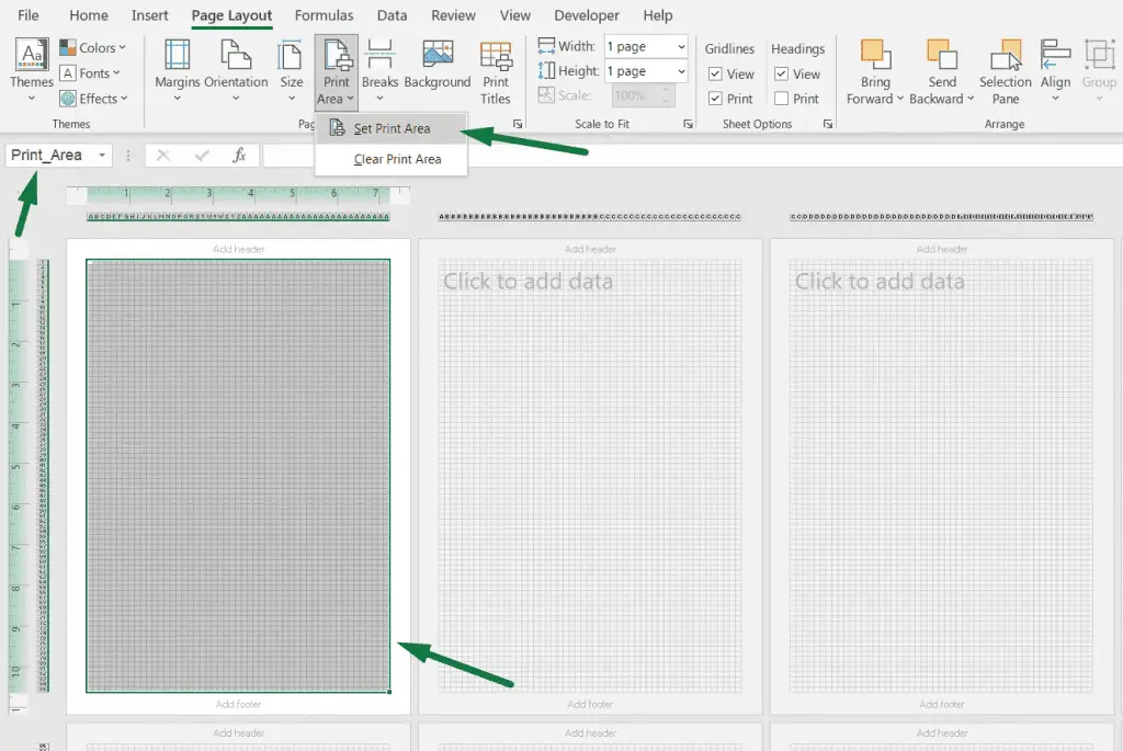
Click on the ‘Print Area’ and select the ‘Set Print Area’ option. Or use this shortcut to set the print area, ‘Alt + P + R + S.’

You will see the ‘Print_Area’ in the name box.

Our sheet is ready to save as a pdf or print the graph paper. 

Step 7: Graph Paper to Print or Save

Click on the ‘Home’ ribbon.  Then select the print option. Or you can press ‘Ctrl +  P,’ which is a shortcut to go to the ‘Print’ section.

You will see this as a preview.

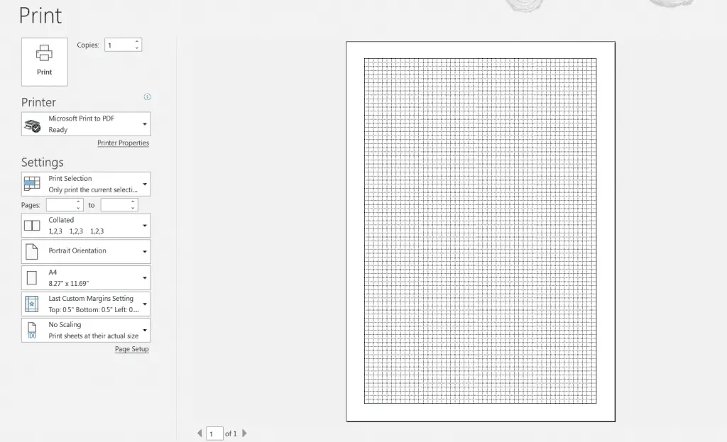
Select your preferred settings and hit the print button to print the graph paper. Similarly, you can also print any chart or graph.

Or, if you wish, you can save it by going to the ‘Save As’ section, selecting the ‘PDF’ option, and then saving it.

Summary

Make graph paper in Excel (With shortcut):

1. Select any blank cell > Press “Ctrl + A.”
2. Press ‘Alt + H + O + H’ to open the column height and input 9.
3. Again, press ‘Alt + H + O + W’ to open the row width tab and input 1.
4. Press “Ctrl + P + PG” to enable the print gridlines option. 
5. Hit ‘Alt + P + M + A’ to open the ‘Custom Margins’ tab, change all the margins to .5, and set the header and footer to 0.
6. Press “Ctrl + P + SZ” to open the paper size and select the “A4” size.
7. Select the ‘Page Layout’ option at the right-bottom corner and make the zoom button 40%. Then, select all the cells on the first page.
8. Hit “Ctrl + P” to go to the print option.

Shortcut Used

1. Select all the cells in a sheet: Ctrl + A or Ctrl + A + A.
2. Open the column height tab: Alt + H + O + H.
3. Open the row width tab: Alt + H + O + W.
4. Enable the print gridlines option: Ctrl + P + PG.
5. Open the ‘Custom Margins’ tab: Alt + P + M + A.
6. Go to the ‘Print’ option: Ctrl + P.

Final Words

We learned how to make graph paper in Excel in many ways. As a bonus, I introduced tons of shortcuts that can make your work process more efficient and effective.

Whether you’re making a graph or drawing a graph paper using Excel, you can do that easily. Let us know if you have any queries regarding making any graph in Excel. 

Happy Learning!